IChO 2007 · Theory problem 1
Proton tunneling
Proton tunneling through energy barriers is an important effect, which can be observed in many complex species containing hydrogen bonds (DNA, proteins, etc.). Propanedial (malonaldehyde) is one of the simplest molecules for which intramolecular proton transfer can occur.
1.1 Draw the condensed formula of propanedial and the structures of two of its isomers, which can exist in equilibrium with propanedial.
1.2 In a water solution propanedial is a weak acid, its strength being comparable with that of acetic acid. Specify the acidic hydrogen atom. Explain its acidity (choose one version in the Answer Sheet).
On the plot below an energy profile of the intramolecular proton transfer is given (the dependence of energy on the distance of proton motion (in nm)). Energy curve has a symmetric double-well form.
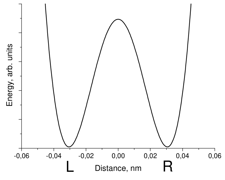
1.3 Draw the structures corresponding to two minima on this curve.
A proton is delocalized between two atoms and oscillates between two minima L and R with an angular frequency \(\omega = 6.48\times10^{11}\ \mathrm{s^{-1}}\). Probability density for a proton depends on time as follows:
\[ \Psi^{2}(x,t)=\frac{1}{2}\left[ \Psi_{\mathrm L}^{2}(x)+\Psi_{\mathrm R}^{2}(x) +\left(\Psi_{\mathrm L}^{2}(x)-\Psi_{\mathrm R}^{2}(x)\right) \cos(\omega t) \right], \]
wavefunctions \(\Psi_{\mathrm L}(x)\) and \(\Psi_{\mathrm R}(x)\) describe a proton localized in the left and right wells, respectively:
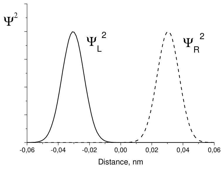
1.4 Write down the expressions for the probability density at three moments: (a) \(t = 0\), (b) \(t = \pi/(2\omega)\), (c) \(t = \pi/\omega\). Sketch the graphs of these three functions.
1.5 Without calculations, determine the probability of finding the proton in the left well at \(t = \pi/(2\omega)\)
1.6 How much time is required for a proton to move from one well to another? What is the proton mean speed during the transfer?
1.7 From the energy curve, estimate the uncertainty of the position of proton forming hydrogen bonds. Estimate the minimal uncertainty of the proton speed. Compare this value with that obtained in 1.6 and draw a conclusion about the proton tunneling (choose one of the versions in the Answer Sheet).
Official English text of the problem.
Answers
-
1.1: Propanedial (malonaldehyde), \(\ce{OHC-CH2-CHO}\), SMILES
O=CCC=O. Its two geometrical enol isomers are (Z)-3-hydroxyprop-2-enal,O=C/C=C\O, and (E)-3-hydroxyprop-2-enal,O=C/C=C/O. -
1.2: Either equivalent hydrogen on the central \(\ce{CH2}\) group can undergo the first dissociation. In the enol form, the corresponding acidic hydrogen is on \(\ce{OH}\). The conjugate base, propanedial enolate,
O=C[CH-]C=O, is stabilized by delocalization of negative charge over both carbonyl groups. -
1.3: The minima are two equivalent, internally hydrogen-bonded arrangements of (Z)-3-hydroxyprop-2-enal: L,
O/C=C\C=O, and R,O=C/C=C\O. With the heavy-atom skeleton held fixed, the proton is bonded to the left oxygen in L and the right oxygen in R; the double bonds shift accordingly. -
1.4:
(a) \(\displaystyle \Psi^{2}(x,0)=\Psi_{\mathrm L}^{2}(x)\): the left peak.
(b) \(\displaystyle \Psi^{2}\!\left(x,\frac{\pi}{2\omega}\right)=\frac12\left[\Psi_{\mathrm L}^{2}(x)+\Psi_{\mathrm R}^{2}(x)\right]\): two equal peaks, each scaled by one-half.
(c) \(\displaystyle \Psi^{2}\!\left(x,\frac{\pi}{\omega}\right)=\Psi_{\mathrm R}^{2}(x)\): the right peak. -
1.5: \(\boxed{P_{\mathrm L}=1/2=50\%}\).
-
1.6: \(\boxed{t_{\mathrm{transfer}}=4.85\times10^{-12}\ \mathrm{s}=4.85\ \mathrm{ps}}\); the mean transfer speed estimated from the graph is \(\boxed{\bar v\approx12\ \mathrm{m\,s^{-1}}}\).
-
1.7: Using the full separation as the position-uncertainty scale, \(\Delta x\sim0.060\ \mathrm{nm}\), gives \(\boxed{\Delta v_{\min}\sim5.3\times10^{2}\ \mathrm{m\,s^{-1}}}\), about 40 times the mean transfer speed. A strict rms estimate for two narrow, equally populated peaks gives approximately \(1.1\times10^{3}\ \mathrm{m\,s^{-1}}\). Thus a sharply defined classical velocity and trajectory cannot describe this tunneling transfer.
Solution
1.1 — Propanedial and its enol isomers
Propanedial contains an aldehyde group at each end of a three-carbon chain:
\[ \boxed{\ce{OHC-CH2-CHO}}. \]
Its name is propanedial, also called malonaldehyde, and its SMILES is O=CCC=O.
An aldehyde group can undergo keto–enol tautomerization using a hydrogen from the central carbon:
\[ \ce{OHC-CH2-CHO <=> OHC-CH=CH-OH}. \]
The product, 3-hydroxyprop-2-enal, has two different substituents on each carbon of its carbon–carbon double bond, so it has two geometrical isomers:
| Isomer | SMILES | Required drawing |
|---|---|---|
| (Z)-3-hydroxyprop-2-enal | O=C/C=C\O |
Put the \(\ce{CHO}\) and \(\ce{OH}\) substituents on the same side of the carbon–carbon double bond. |
| (E)-3-hydroxyprop-2-enal | O=C/C=C/O |
Put the \(\ce{CHO}\) and \(\ce{OH}\) substituents on opposite sides of the carbon–carbon double bond. |
Both can interconvert with propanedial by tautomerization. Enolization at opposite ends of the symmetrical starting molecule does not produce additional distinct constitutional isomers.
1.2 — Acidic hydrogen and stabilization of the conjugate base
In the dialdehyde structure, identify a hydrogen on the central \(\ce{CH2}\) carbon. The two hydrogens are equivalent before dissociation; loss of either gives the same conjugate base.
The aqueous dissociation can be represented as
\[ \ce{OHC-CH2-CHO + H2O <=> [OHC-CH-CHO]^- + H3O+}. \]
Here water has SMILES O, hydronium has SMILES [OH3+], and the anion is propanedial enolate, represented by O=C[CH-]C=O.
The anion has three principal resonance contributors:
| Location of formal negative charge | SMILES of the contributor |
|---|---|
| Central carbon | O=C[CH-]C=O |
| Left oxygen | [O-]C=CC=O |
| Right oxygen | O=CC=C[O-] |
These are representations of the same delocalized ion, not separate species in equilibrium. The negative charge is distributed over a conjugated framework containing both carbonyl groups, with important contributions placing it on electronegative oxygen atoms. This stabilizes the conjugate base and accounts for the acidity.
In the enol tautomer, removal of the hydroxyl hydrogen produces the same delocalized conjugate base. Thus the acidic site is described as a central-carbon hydrogen in the dialdehyde form and the hydroxyl hydrogen in the enol form.
1.3 — Structures at the two minima
The proton transfers between the two oxygens of the internally hydrogen-bonded (Z)-3-hydroxyprop-2-enal.
Read the following structures with the oxygen–carbon–carbon–carbon–oxygen skeleton held in the same spatial orientation:
| Minimum | Condensed structure | Name and SMILES |
|---|---|---|
| L | \(\ce{HO-CH=CH-CHO}\) | (Z)-3-hydroxyprop-2-enal, O/C=C\C=O |
| R | \(\ce{OHC-CH=CH-OH}\) | (Z)-3-hydroxyprop-2-enal, O=C/C=C\O |
For the drawing, bend the approximately planar chain so that the two oxygens face each other, forming a six-membered hydrogen-bonded loop that includes the transferred hydrogen.
- L: Draw a covalent bond from the left oxygen to hydrogen and a dotted hydrogen bond to the right oxygen: \(\ce{O-H}\cdots\ce{O}\). The left carbon–oxygen bond is single, and the right one is double.
- R: Draw the hydrogen covalently bonded to the right oxygen, with a dotted bond to the left: \(\ce{O}\cdots\ce{H-O}\). The left carbon–oxygen bond is double, and the right one is single.
The carbon–carbon double bond shifts at the same time. The SMILES encode connectivity and alkene geometry, but the inward-facing conformation and dotted hydrogen bond must be shown separately.
The two arrangements are symmetry-equivalent, explaining the equal depths of the wells. They are not the E and Z isomers from part 1.1.
1.4 — Probability densities and sketches
Rewrite the given expression using the half-angle identities:
\[ \Psi^{2}(x,t) = \cos^{2}\!\left(\frac{\omega t}{2}\right)\Psi_{\mathrm L}^{2}(x) + \sin^{2}\!\left(\frac{\omega t}{2}\right)\Psi_{\mathrm R}^{2}(x). \]
(a) At \(t=0\):
\[ \boxed{\Psi^{2}(x,0)=\Psi_{\mathrm L}^{2}(x)}. \]
Draw the supplied left-hand peak, centered at approximately \(-0.030\ \mathrm{nm}\), with its original shape and height.
(b) At \(t=\pi/(2\omega)\):
Since \(\cos(\omega t)=\cos(\pi/2)=0\),
\[ \boxed{ \Psi^{2}\!\left(x,\frac{\pi}{2\omega}\right) = \frac12\Psi_{\mathrm L}^{2}(x) + \frac12\Psi_{\mathrm R}^{2}(x) }. \]
Draw two equal peaks centered at approximately \(-0.030\) and \(+0.030\ \mathrm{nm}\). Each component has the original width but half its original height and integrated area \(1/2\).
(c) At \(t=\pi/\omega\):
Since \(\cos(\omega t)=\cos\pi=-1\),
\[ \boxed{ \Psi^{2}\!\left(x,\frac{\pi}{\omega}\right) =\Psi_{\mathrm R}^{2}(x) }. \]
Draw the supplied right-hand peak, centered at approximately \(+0.030\ \mathrm{nm}\), with its original shape and height.
1.5 — Probability in the left well
At \(t=\pi/(2\omega)\), the density is symmetric between the two wells. The total probability is one, so each well has probability
\[ \boxed{P_{\mathrm L}=\frac12}. \]
1.6 — Transfer time and mean speed
The proton starts in the left-localized state at \(t=0\) and first reaches the right-localized state when \(\omega t=\pi\). Therefore,
\[ t_{\mathrm{transfer}} =\frac{\pi}{\omega} =\frac{\pi}{6.48\times10^{11}\ \mathrm{s^{-1}}} =\boxed{4.85\times10^{-12}\ \mathrm{s}}. \]
This is half the oscillation period.
From the graph, the minima are approximately at \(-0.030\) and \(+0.030\ \mathrm{nm}\), so their separation is
\[ d=0.060\ \mathrm{nm}=6.0\times10^{-11}\ \mathrm{m}. \]
The requested distance-over-time estimate is
\[ \bar v =\frac{d}{t_{\mathrm{transfer}}} =\frac{6.0\times10^{-11}\ \mathrm{m}} {4.848\times10^{-12}\ \mathrm{s}} =12.4\ \mathrm{m\,s^{-1}} \approx\boxed{12\ \mathrm{m\,s^{-1}}}. \]
The precision is limited by reading the distance from the graph.
1.7 — Position and velocity uncertainties
The graph gives a characteristic proton-delocalization distance of
\[ \Delta x\sim d=0.060\ \mathrm{nm}=6.0\times10^{-11}\ \mathrm{m}. \]
Use the position–momentum uncertainty relation,
\[ \Delta x\,\Delta p_x\ge\frac{\hbar}{2}, \]
and, for a nonrelativistic proton, \(\Delta p_x=m_p\Delta v_x\). Hence,
\[ \Delta v_x\ge\frac{\hbar}{2m_p\Delta x}. \]
Using the standard constants
\[ \hbar=1.055\times10^{-34}\ \mathrm{J\,s}, \qquad m_p=1.673\times10^{-27}\ \mathrm{kg}, \]
the graph-based estimate is
\[ \Delta v_{\min} \sim \frac{1.055\times10^{-34}} {2(1.673\times10^{-27})(6.0\times10^{-11})} = \boxed{5.3\times10^{2}\ \mathrm{m\,s^{-1}}}. \]
Compared with part 1.6,
\[ \frac{\Delta v_{\min}}{\bar v} \approx\frac{525}{12.4} \approx42. \]
There is a factor-of-two convention to distinguish here. In the exact uncertainty relation, \(\Delta x\) denotes a standard deviation, rather than a full spatial span. At equal populations, two narrow peaks centered at \(\pm0.030\ \mathrm{nm}\) have a position standard deviation approximately \(0.030\ \mathrm{nm}\). That estimate gives
\[ \Delta v_{\min}\sim1.1\times10^{3}\ \mathrm{m\,s^{-1}}, \]
which leads to the same conclusion.
The velocity uncertainty is much larger than the distance-over-time speed. Thus part 1.6 supplies a characteristic transfer speed, but it does not establish a classical trajectory with a sharply defined velocity through the barrier. The transfer requires a quantum-mechanical description.
The solution was checked against the official solution.
IChO 2007 · Theorieaufgabe 1
Protonentunneln
Das Tunneln von Protonen durch Energiebarrieren ist ein wichtiger Effekt, der in vielen komplexen Spezies mit Wasserstoffbrückenbindungen (DNA, Proteine usw.) beobachtet werden kann. Propandial (Malonaldehyd) ist eines der einfachsten Moleküle, bei denen ein intramolekularer Protonentransfer auftreten kann.
1.1 Zeichnen Sie die Halbstrukturformel von Propandial und die Strukturen zweier seiner Isomere, die mit Propandial im Gleichgewicht vorliegen können.
1.2 In wässriger Lösung ist Propandial eine schwache Säure, deren Stärke mit der von Essigsäure vergleichbar ist. Geben Sie das saure Wasserstoffatom an. Erklären Sie seine Acidität (wählen Sie eine Antwortmöglichkeit auf dem Antwortbogen).
In der folgenden Abbildung ist ein Energieprofil des intramolekularen Protonentransfers dargestellt (die Abhängigkeit der Energie von der Strecke der Protonenbewegung (in nm)). Die Energiekurve hat die Form eines symmetrischen Doppelmuldenpotentials.
1.3 Zeichnen Sie die Strukturen, die den beiden Minima dieser Kurve entsprechen.
Ein Proton ist zwischen zwei Atomen delokalisiert und oszilliert zwischen zwei Minima L und R mit einer Kreisfrequenz von \(\omega = 6.48\times10^{11}\ \mathrm{s^{-1}}\). Die Wahrscheinlichkeitsdichte für ein Proton hängt wie folgt von der Zeit ab:
\[ \Psi^{2}(x,t)=\frac{1}{2}\left[ \Psi_{\mathrm L}^{2}(x)+\Psi_{\mathrm R}^{2}(x) +\left(\Psi_{\mathrm L}^{2}(x)-\Psi_{\mathrm R}^{2}(x)\right) \cos(\omega t) \right], \]
wobei die Wellenfunktionen \(\Psi_{\mathrm L}(x)\) und \(\Psi_{\mathrm R}(x)\) ein in der linken bzw. rechten Potentialmulde lokalisiertes Proton beschreiben:
1.4 Geben Sie die Ausdrücke für die Wahrscheinlichkeitsdichte zu drei Zeitpunkten an: (a) \(t = 0\), (b) \(t = \pi/(2\omega)\), (c) \(t = \pi/\omega\). Skizzieren Sie die Graphen dieser drei Funktionen.
1.5 Bestimmen Sie ohne Rechnung die Wahrscheinlichkeit, das Proton bei \(t = \pi/(2\omega)\) in der linken Potentialmulde zu finden.
1.6 Wie viel Zeit benötigt ein Proton, um sich von einer Potentialmulde zur anderen zu bewegen? Wie groß ist die mittlere Geschwindigkeit des Protons während des Transfers?
1.7 Schätzen Sie anhand der Energiekurve die Ortsunschärfe des Protons ab, das Wasserstoffbrückenbindungen bildet. Schätzen Sie die minimale Geschwindigkeitsunschärfe des Protons ab. Vergleichen Sie diesen Wert mit dem in 1.6 erhaltenen Wert und ziehen Sie eine Schlussfolgerung zum Protonentunneln (wählen Sie eine der Antwortmöglichkeiten auf dem Antwortbogen).
Aufgabentext aus dem offiziellen englischen Text übersetzt.
Antworten
-
1.1: Propandial (Malonaldehyd), \(\ce{OHC-CH2-CHO}\), SMILES
O=CCC=O. Seine beiden geometrischen Enolisomere sind (Z)-3-Hydroxyprop-2-enal,O=C/C=C\O, und (E)-3-Hydroxyprop-2-enal,O=C/C=C/O. -
1.2: Jedes der beiden äquivalenten Wasserstoffatome an der zentralen \(\ce{CH2}\)-Gruppe kann bei der ersten Dissoziation abgespalten werden. In der Enolform befindet sich das entsprechende saure Wasserstoffatom an \(\ce{OH}\). Die konjugierte Base, das Propandial-Enolat,
O=C[CH-]C=O, wird durch Delokalisierung der negativen Ladung über beide Carbonylgruppen stabilisiert. -
1.3: Die Minima sind zwei äquivalente Anordnungen von (Z)-3-Hydroxyprop-2-enal mit einer intramolekularen Wasserstoffbrückenbindung: L,
O/C=C\C=O, und R,O=C/C=C\O. Bei festgehaltenem Gerüst der schweren Atome ist das Proton in L an das linke und in R an das rechte Sauerstoffatom gebunden; die Doppelbindungen verschieben sich entsprechend. -
1.4:
(a) \(\displaystyle \Psi^{2}(x,0)=\Psi_{\mathrm L}^{2}(x)\): der linke Peak.
(b) \(\displaystyle \Psi^{2}\!\left(x,\frac{\pi}{2\omega}\right)=\frac12\left[\Psi_{\mathrm L}^{2}(x)+\Psi_{\mathrm R}^{2}(x)\right]\): zwei gleich große Peaks, jeweils mit dem Faktor ein halb skaliert.
(c) \(\displaystyle \Psi^{2}\!\left(x,\frac{\pi}{\omega}\right)=\Psi_{\mathrm R}^{2}(x)\): der rechte Peak. -
1.5: \(\boxed{P_{\mathrm L}=1/2=50\%}\).
-
1.6: \(\boxed{t_{\mathrm{transfer}}=4.85\times10^{-12}\ \mathrm{s}=4.85\ \mathrm{ps}}\); die anhand des Graphen geschätzte mittlere Transfergeschwindigkeit beträgt \(\boxed{\bar v\approx12\ \mathrm{m\,s^{-1}}}\).
-
1.7: Verwendet man den gesamten Abstand als Maß für die Ortsunschärfe, \(\Delta x\sim0.060\ \mathrm{nm}\), erhält man \(\boxed{\Delta v_{\min}\sim5.3\times10^{2}\ \mathrm{m\,s^{-1}}}\), etwa das 40-Fache der mittleren Transfergeschwindigkeit. Eine strenge Abschätzung anhand der Standardabweichung für zwei schmale, gleich besetzte Peaks ergibt etwa \(1.1\times10^{3}\ \mathrm{m\,s^{-1}}\). Somit können eine scharf definierte klassische Geschwindigkeit und Bahn diesen Tunneltransfer nicht beschreiben.
Lösung
1.1 — Propandial und seine Enolisomere
Propandial enthält an jedem Ende einer Kette aus drei Kohlenstoffatomen eine Aldehydgruppe:
\[ \boxed{\ce{OHC-CH2-CHO}}. \]
Sein Name ist Propandial, auch Malonaldehyd genannt, und sein SMILES lautet O=CCC=O.
Eine Aldehydgruppe kann unter Beteiligung eines Wasserstoffatoms am zentralen Kohlenstoffatom eine Keto-Enol-Tautomerisierung eingehen:
\[ \ce{OHC-CH2-CHO <=> OHC-CH=CH-OH}. \]
Das Produkt, 3-Hydroxyprop-2-enal, besitzt an jedem Kohlenstoffatom seiner Kohlenstoff-Kohlenstoff-Doppelbindung zwei verschiedene Substituenten und hat daher zwei geometrische Isomere:
| Isomer | SMILES | Geforderte Zeichnung |
|---|---|---|
| (Z)-3-Hydroxyprop-2-enal | O=C/C=C\O |
Ordnen Sie die Substituenten \(\ce{CHO}\) und \(\ce{OH}\) auf derselben Seite der Kohlenstoff-Kohlenstoff-Doppelbindung an. |
| (E)-3-Hydroxyprop-2-enal | O=C/C=C/O |
Ordnen Sie die Substituenten \(\ce{CHO}\) und \(\ce{OH}\) auf entgegengesetzten Seiten der Kohlenstoff-Kohlenstoff-Doppelbindung an. |
Beide können durch Tautomerisierung in Propandial übergehen und umgekehrt. Eine Enolisierung an den entgegengesetzten Enden des symmetrischen Ausgangsmoleküls erzeugt keine weiteren unterschiedlichen Konstitutionsisomere.
1.2 — Saures Wasserstoffatom und Stabilisierung der konjugierten Base
Markieren Sie in der Dialdehydstruktur ein Wasserstoffatom am zentralen \(\ce{CH2}\)-Kohlenstoffatom. Die beiden Wasserstoffatome sind vor der Dissoziation äquivalent; die Abspaltung eines beliebigen der beiden ergibt dieselbe konjugierte Base.
Die Dissoziation in wässriger Lösung lässt sich folgendermaßen darstellen:
\[ \ce{OHC-CH2-CHO + H2O <=> [OHC-CH-CHO]^- + H3O+}. \]
Hier hat Wasser den SMILES O, das Oxoniumion den SMILES [OH3+], und das Anion ist das Propandial-Enolat, dargestellt durch O=C[CH-]C=O.
Das Anion besitzt drei wesentliche mesomere Grenzstrukturen:
| Ort der formalen negativen Ladung | SMILES der Grenzstruktur |
|---|---|
| Zentrales Kohlenstoffatom | O=C[CH-]C=O |
| Linkes Sauerstoffatom | [O-]C=CC=O |
| Rechtes Sauerstoffatom | O=CC=C[O-] |
Dies sind Darstellungen desselben delokalisierten Ions, keine getrennten, miteinander im Gleichgewicht stehenden Spezies. Die negative Ladung ist über ein konjugiertes Gerüst verteilt, das beide Carbonylgruppen umfasst; wesentliche Beiträge stammen von Grenzstrukturen, in denen sie an elektronegativen Sauerstoffatomen sitzt. Dies stabilisiert die konjugierte Base und erklärt die Acidität.
Im Enoltautomer führt die Abspaltung des Hydroxylwasserstoffatoms zur selben delokalisierten konjugierten Base. Die saure Stelle wird somit in der Dialdehydform als ein Wasserstoffatom am zentralen Kohlenstoffatom und in der Enolform als das Hydroxylwasserstoffatom beschrieben.
1.3 — Strukturen an den beiden Minima
Das Proton wird zwischen den beiden Sauerstoffatomen des (Z)-3-Hydroxyprop-2-enals mit seiner intramolekularen Wasserstoffbrückenbindung übertragen.
Lesen Sie die folgenden Strukturen so, dass das Sauerstoff-Kohlenstoff-Kohlenstoff-Kohlenstoff-Sauerstoff-Gerüst in derselben räumlichen Orientierung festgehalten wird:
| Minimum | Halbstrukturformel | Name und SMILES |
|---|---|---|
| L | \(\ce{HO-CH=CH-CHO}\) | (Z)-3-Hydroxyprop-2-enal, O/C=C\C=O |
| R | \(\ce{OHC-CH=CH-OH}\) | (Z)-3-Hydroxyprop-2-enal, O=C/C=C\O |
Krümmen Sie für die Zeichnung die annähernd ebene Kette so, dass die beiden Sauerstoffatome einander zugewandt sind und einen durch eine Wasserstoffbrückenbindung geschlossenen sechsgliedrigen Ring bilden, der das übertragene Wasserstoffatom einschließt.
- L: Zeichnen Sie eine kovalente Bindung vom linken Sauerstoffatom zum Wasserstoffatom und eine gepunktete Wasserstoffbrückenbindung zum rechten Sauerstoffatom: \(\ce{O-H}\cdots\ce{O}\). Die linke Kohlenstoff-Sauerstoff-Bindung ist eine Einfachbindung, die rechte eine Doppelbindung.
- R: Zeichnen Sie das Wasserstoffatom kovalent an das rechte Sauerstoffatom gebunden, mit einer gepunkteten Bindung zum linken: \(\ce{O}\cdots\ce{H-O}\). Die linke Kohlenstoff-Sauerstoff-Bindung ist eine Doppelbindung, die rechte eine Einfachbindung.
Die Kohlenstoff-Kohlenstoff-Doppelbindung verschiebt sich gleichzeitig. Die SMILES kodieren die Konnektivität und die Alkengeometrie, aber die nach innen gerichtete Konformation und die gepunktete Wasserstoffbrückenbindung müssen gesondert dargestellt werden.
Die beiden Anordnungen sind symmetrieäquivalent, was die gleiche Tiefe der Potentialmulden erklärt. Es handelt sich nicht um die E- und Z-Isomere aus Teil 1.1.
1.4 — Wahrscheinlichkeitsdichten und Skizzen
Schreiben Sie den gegebenen Ausdruck mithilfe der Halbwinkelformeln um:
\[ \Psi^{2}(x,t) = \cos^{2}\!\left(\frac{\omega t}{2}\right)\Psi_{\mathrm L}^{2}(x) + \sin^{2}\!\left(\frac{\omega t}{2}\right)\Psi_{\mathrm R}^{2}(x). \]
(a) Bei \(t=0\):
\[ \boxed{\Psi^{2}(x,0)=\Psi_{\mathrm L}^{2}(x)}. \]
Zeichnen Sie den vorgegebenen linken Peak mit seinem Zentrum bei etwa \(-0.030\ \mathrm{nm}\) und mit seiner ursprünglichen Form und Höhe.
(b) Bei \(t=\pi/(2\omega)\):
Da \(\cos(\omega t)=\cos(\pi/2)=0\), gilt
\[ \boxed{ \Psi^{2}\!\left(x,\frac{\pi}{2\omega}\right) = \frac12\Psi_{\mathrm L}^{2}(x) + \frac12\Psi_{\mathrm R}^{2}(x) }. \]
Zeichnen Sie zwei gleich große Peaks mit ihren Zentren bei etwa \(-0.030\) und \(+0.030\ \mathrm{nm}\). Jede Komponente hat die ursprüngliche Breite, aber die Hälfte ihrer ursprünglichen Höhe und eine integrierte Fläche von \(1/2\).
(c) Bei \(t=\pi/\omega\):
Da \(\cos(\omega t)=\cos\pi=-1\), gilt
\[ \boxed{ \Psi^{2}\!\left(x,\frac{\pi}{\omega}\right) =\Psi_{\mathrm R}^{2}(x) }. \]
Zeichnen Sie den vorgegebenen rechten Peak mit seinem Zentrum bei etwa \(+0.030\ \mathrm{nm}\) und mit seiner ursprünglichen Form und Höhe.
1.5 — Wahrscheinlichkeit in der linken Potentialmulde
Bei \(t=\pi/(2\omega)\) ist die Dichte bezüglich der beiden Potentialmulden symmetrisch. Die Gesamtwahrscheinlichkeit beträgt eins, sodass für jede Potentialmulde folgende Wahrscheinlichkeit gilt:
\[ \boxed{P_{\mathrm L}=\frac12}. \]
1.6 — Transferzeit und mittlere Geschwindigkeit
Das Proton startet bei \(t=0\) im links lokalisierten Zustand und erreicht den rechts lokalisierten Zustand erstmals, wenn \(\omega t=\pi\). Daher gilt
\[ t_{\mathrm{transfer}} =\frac{\pi}{\omega} =\frac{\pi}{6.48\times10^{11}\ \mathrm{s^{-1}}} =\boxed{4.85\times10^{-12}\ \mathrm{s}}. \]
Dies ist die Hälfte der Schwingungsdauer.
Dem Graphen zufolge liegen die Minima ungefähr bei \(-0.030\) und \(+0.030\ \mathrm{nm}\), sodass ihr Abstand beträgt:
\[ d=0.060\ \mathrm{nm}=6.0\times10^{-11}\ \mathrm{m}. \]
Die geforderte Abschätzung als Quotient aus Strecke und Zeit ergibt
\[ \bar v =\frac{d}{t_{\mathrm{transfer}}} =\frac{6.0\times10^{-11}\ \mathrm{m}} {4.848\times10^{-12}\ \mathrm{s}} =12.4\ \mathrm{m\,s^{-1}} \approx\boxed{12\ \mathrm{m\,s^{-1}}}. \]
Die Genauigkeit ist durch das Ablesen des Abstands aus dem Graphen begrenzt.
1.7 — Orts- und Geschwindigkeitsunschärfen
Der Graph liefert eine charakteristische Delokalisierungsstrecke des Protons von
\[ \Delta x\sim d=0.060\ \mathrm{nm}=6.0\times10^{-11}\ \mathrm{m}. \]
Verwenden Sie die Ort-Impuls-Unschärferelation,
\[ \Delta x\,\Delta p_x\ge\frac{\hbar}{2}, \]
und für ein nichtrelativistisches Proton \(\Delta p_x=m_p\Delta v_x\). Daraus folgt
\[ \Delta v_x\ge\frac{\hbar}{2m_p\Delta x}. \]
Mit den üblichen Konstanten
\[ \hbar=1.055\times10^{-34}\ \mathrm{J\,s}, \qquad m_p=1.673\times10^{-27}\ \mathrm{kg}, \]
ergibt die Abschätzung anhand des Graphen
\[ \Delta v_{\min} \sim \frac{1.055\times10^{-34}} {2(1.673\times10^{-27})(6.0\times10^{-11})} = \boxed{5.3\times10^{2}\ \mathrm{m\,s^{-1}}}. \]
Im Vergleich mit Teil 1.6 gilt
\[ \frac{\Delta v_{\min}}{\bar v} \approx\frac{525}{12.4} \approx42. \]
Hier ist ein konventionsbedingter Faktor zwei zu beachten. In der exakten Unschärferelation bezeichnet \(\Delta x\) eine Standardabweichung und nicht eine gesamte räumliche Ausdehnung. Bei gleicher Besetzung haben zwei schmale Peaks mit ihren Zentren bei \(\pm0.030\ \mathrm{nm}\) eine Ortsstandardabweichung von ungefähr \(0.030\ \mathrm{nm}\). Diese Abschätzung ergibt
\[ \Delta v_{\min}\sim1.1\times10^{3}\ \mathrm{m\,s^{-1}}, \]
was zur selben Schlussfolgerung führt.
Die Geschwindigkeitsunschärfe ist viel größer als die aus Strecke und Zeit ermittelte Geschwindigkeit. Teil 1.6 liefert somit eine charakteristische Transfergeschwindigkeit, legt aber keine klassische Bahn mit einer scharf definierten Geschwindigkeit durch die Barriere fest. Der Transfer erfordert eine quantenmechanische Beschreibung.
Die Lösung wurde mit der offiziellen Lösung abgeglichen.
IChO 2007 · Teori sorusu 1
Proton tünellemesi
Protonların enerji engellerinden tünelleme yoluyla geçmesi, hidrojen bağları içeren birçok karmaşık türde (DNA, proteinler vb.) gözlenebilen önemli bir etkidir. Propandial (malonaldehit), molekül içi proton aktarımının gerçekleşebildiği en basit moleküllerden biridir.
1.1 Propandialin yoğunlaştırılmış formülünü ve propandial ile dengede bulunabilen iki izomerinin yapılarını çiziniz.
1.2 Propandial, sulu çözeltide asitliği asetik asidinkiyle karşılaştırılabilir düzeyde olan zayıf bir asittir. Asidik hidrojen atomunu belirtiniz. Asitliğini açıklayınız (Cevap Kâğıdı'ndaki seçeneklerden birini seçiniz).
Aşağıdaki grafikte molekül içi proton aktarımının enerji profili (enerjinin protonun hareket mesafesine (nm cinsinden) bağlılığı) verilmiştir. Enerji eğrisi simetrik bir çift kuyu biçimindedir.
1.3 Bu eğrideki iki minimuma karşılık gelen yapıları çiziniz.
Bir proton iki atom arasında delokalizedir ve L ile R minimumları arasında \(\omega = 6.48\times10^{11}\ \mathrm{s^{-1}}\) açısal frekansıyla salınım yapar. Protonun olasılık yoğunluğu zamana aşağıdaki gibi bağlıdır:
\[ \Psi^{2}(x,t)=\frac{1}{2}\left[ \Psi_{\mathrm L}^{2}(x)+\Psi_{\mathrm R}^{2}(x) +\left(\Psi_{\mathrm L}^{2}(x)-\Psi_{\mathrm R}^{2}(x)\right) \cos(\omega t) \right], \]
\(\Psi_{\mathrm L}(x)\) ve \(\Psi_{\mathrm R}(x)\) dalga fonksiyonları, sırasıyla sol ve sağ kuyuda lokalize olmuş bir protonu betimler:
1.4 Üç an için olasılık yoğunluğu ifadelerini yazınız: (a) \(t = 0\), (b) \(t = \pi/(2\omega)\), (c) \(t = \pi/\omega\). Bu üç fonksiyonun grafiklerini kabaca çiziniz.
1.5 Hesaplama yapmadan, \(t = \pi/(2\omega)\) anında protonu sol kuyuda bulma olasılığını belirleyiniz.
1.6 Bir protonun bir kuyudan diğerine geçmesi için ne kadar süre gerekir? Aktarım sırasında protonun ortalama sürati nedir?
1.7 Enerji eğrisinden, hidrojen bağları oluşturan protonun konum belirsizliğini tahmin ediniz. Protonun süratindeki en küçük belirsizliği tahmin ediniz. Bu değeri 1.6'da elde edilen değerle karşılaştırınız ve proton tünellemesi hakkında bir sonuca varınız (Cevap Kâğıdı'ndaki seçeneklerden birini seçiniz).
Soru metni resmi İngilizce metinden çevrilmiştir.
Cevaplar
-
1.1: Propandial (malonaldehit), \(\ce{OHC-CH2-CHO}\), SMILES
O=CCC=O. İki geometrik enol izomeri (Z)-3-hidroksiprop-2-enal,O=C/C=C\O, ve (E)-3-hidroksiprop-2-enal,O=C/C=C/O'dür. -
1.2: Merkezdeki \(\ce{CH2}\) grubunun eşdeğer hidrojenlerinden herhangi biri ilk ayrışmada kopabilir. Enol biçiminde, buna karşılık gelen asidik hidrojen \(\ce{OH}\) üzerindedir. Eşlenik baz olan propandial enolat,
O=C[CH-]C=O, negatif yükün her iki karbonil grubu üzerinde delokalizasyonuyla kararlı hâle gelir. -
1.3: Minimumlar, (Z)-3-hidroksiprop-2-enal molekülünün molekül içi hidrojen bağı içeren iki eşdeğer düzenlenişidir: L,
O/C=C\C=O, ve R,O=C/C=C\O. Ağır atom iskeleti sabit tutulduğunda proton, L'de soldaki oksijene, R'de ise sağdaki oksijene bağlıdır; çift bağlar da buna uygun olarak yer değiştirir. -
1.4:
(a) \(\displaystyle \Psi^{2}(x,0)=\Psi_{\mathrm L}^{2}(x)\): soldaki tepe.
(b) \(\displaystyle \Psi^{2}\!\left(x,\frac{\pi}{2\omega}\right)=\frac12\left[\Psi_{\mathrm L}^{2}(x)+\Psi_{\mathrm R}^{2}(x)\right]\): her biri yarı ölçeğe indirilmiş iki eşit tepe.
(c) \(\displaystyle \Psi^{2}\!\left(x,\frac{\pi}{\omega}\right)=\Psi_{\mathrm R}^{2}(x)\): sağdaki tepe. -
1.5: \(\boxed{P_{\mathrm L}=1/2=50\%}\).
-
1.6: \(\boxed{t_{\mathrm{transfer}}=4.85\times10^{-12}\ \mathrm{s}=4.85\ \mathrm{ps}}\); grafikten tahmin edilen ortalama aktarım sürati \(\boxed{\bar v\approx12\ \mathrm{m\,s^{-1}}}\)'dir.
-
1.7: Konum belirsizliğinin ölçeği olarak aradaki uzaklığın tamamı, \(\Delta x\sim0.060\ \mathrm{nm}\), kullanıldığında \(\boxed{\Delta v_{\min}\sim5.3\times10^{2}\ \mathrm{m\,s^{-1}}}\) elde edilir; bu, ortalama aktarım süratinin yaklaşık 40 katıdır. Eşit olasılık ağırlığına sahip iki dar tepe için kesin tanıma uygun bir karekök ortalama kare (rms) tahmini yaklaşık \(1.1\times10^{3}\ \mathrm{m\,s^{-1}}\) verir. Dolayısıyla kesin olarak belirlenmiş bir klasik hız ve yörünge, bu tünelleme aktarımını betimleyemez.
Çözüm
1.1 — Propandial ve enol izomerleri
Propandial, üç karbonlu bir zincirin her iki ucunda birer aldehit grubu içerir:
\[ \boxed{\ce{OHC-CH2-CHO}}. \]
Adı propandial olup malonaldehit olarak da adlandırılır ve SMILES gösterimi O=CCC=O'dur.
Bir aldehit grubu, merkezdeki karbondan bir hidrojen alarak keto–enol tautomerleşmesine uğrayabilir:
\[ \ce{OHC-CH2-CHO <=> OHC-CH=CH-OH}. \]
Ürün olan 3-hidroksiprop-2-enal, karbon–karbon çift bağının her bir karbonunda iki farklı sübstitüent taşır; bu nedenle iki geometrik izomeri vardır:
| İzomer | SMILES | İstenen çizim |
|---|---|---|
| (Z)-3-hidroksiprop-2-enal | O=C/C=C\O |
\(\ce{CHO}\) ve \(\ce{OH}\) sübstitüentlerini karbon–karbon çift bağının aynı tarafına yerleştiriniz. |
| (E)-3-hidroksiprop-2-enal | O=C/C=C/O |
\(\ce{CHO}\) ve \(\ce{OH}\) sübstitüentlerini karbon–karbon çift bağının karşı taraflarına yerleştiriniz. |
Her ikisi de tautomerleşme yoluyla propandiale dönüşebilir ve propandialden oluşabilir. Simetrik başlangıç molekülünün karşıt uçlarında gerçekleşen enolleşme, ek farklı yapı izomerleri oluşturmaz.
1.2 — Asidik hidrojen ve eşlenik bazın kararlı hâle gelmesi
Dialdehit yapısında, merkezdeki \(\ce{CH2}\) karbonuna bağlı bir hidrojeni belirleyiniz. İki hidrojen ayrışmadan önce eşdeğerdir; hangisi koparsa kopsun aynı eşlenik baz oluşur.
Sulu ortamda ayrışma şöyle gösterilebilir:
\[ \ce{OHC-CH2-CHO + H2O <=> [OHC-CH-CHO]^- + H3O+}. \]
Burada suyun SMILES gösterimi O, hidronyumun SMILES gösterimi [OH3+] olup anyon, O=C[CH-]C=O ile gösterilen propandial enolattır.
Anyonun başlıca üç rezonans katkı yapısı vardır:
| Biçimsel negatif yükün konumu | Katkı yapısının SMILES gösterimi |
|---|---|
| Merkezdeki karbon | O=C[CH-]C=O |
| Soldaki oksijen | [O-]C=CC=O |
| Sağdaki oksijen | O=CC=C[O-] |
Bunlar dengede bulunan ayrı türler değil, aynı delokalize iyonun gösterimleridir. Negatif yük, her iki karbonil grubunu içeren konjuge bir iskelet üzerine dağılmıştır; yükü elektronegatif oksijen atomları üzerine yerleştiren yapıların katkısı önemlidir. Bu durum eşlenik bazı kararlı hâle getirir ve asitliği açıklar.
Enol tautomerinde hidroksil hidrojeninin uzaklaştırılması aynı delokalize eşlenik bazı oluşturur. Dolayısıyla asidik konum, dialdehit biçiminde merkezdeki karbona bağlı bir hidrojen, enol biçiminde ise hidroksil hidrojeni olarak tanımlanır.
1.3 — İki minimumdaki yapılar
Proton, molekül içi hidrojen bağı içeren (Z)-3-hidroksiprop-2-enal molekülünün iki oksijeni arasında aktarılır.
Aşağıdaki yapıları, oksijen–karbon–karbon–karbon–oksijen iskeletinin uzaydaki yönelimi aynı tutulmuş olarak okuyunuz:
| Minimum | Yoğunlaştırılmış yapı | Adı ve SMILES gösterimi |
|---|---|---|
| L | \(\ce{HO-CH=CH-CHO}\) | (Z)-3-hidroksiprop-2-enal, O/C=C\C=O |
| R | \(\ce{OHC-CH=CH-OH}\) | (Z)-3-hidroksiprop-2-enal, O=C/C=C\O |
Çizimde, yaklaşık olarak düzlemsel olan zinciri iki oksijen birbirine bakacak şekilde bükünüz; böylece aktarılan hidrojeni de içeren, hidrojen bağıyla kapanan altı üyeli bir halka oluşur.
- L: Soldaki oksijenden hidrojene bir kovalent bağ ve sağdaki oksijene noktalı bir hidrojen bağı çiziniz: \(\ce{O-H}\cdots\ce{O}\). Soldaki karbon–oksijen bağı tek, sağdaki ise çifttir.
- R: Hidrojeni sağdaki oksijene kovalent bağla bağlı, soldaki oksijene ise noktalı bağla bağlı olarak çiziniz: \(\ce{O}\cdots\ce{H-O}\). Soldaki karbon–oksijen bağı çift, sağdaki ise tektir.
Karbon–karbon çift bağı da aynı anda yer değiştirir. SMILES gösterimleri atomların bağlanma düzenini ve alken geometrisini kodlar; ancak içe dönük konformasyon ve noktalı hidrojen bağı ayrıca gösterilmelidir.
İki düzenleniş simetri bakımından eşdeğerdir; bu da kuyuların derinliklerinin eşit olmasını açıklar. Bunlar, 1.1 kısmındaki E ve Z izomerleri değildir.
1.4 — Olasılık yoğunlukları ve grafiklerin çizimi
Verilen ifadeyi yarım açı özdeşliklerini kullanarak yeniden yazınız:
\[ \Psi^{2}(x,t) = \cos^{2}\!\left(\frac{\omega t}{2}\right)\Psi_{\mathrm L}^{2}(x) + \sin^{2}\!\left(\frac{\omega t}{2}\right)\Psi_{\mathrm R}^{2}(x). \]
(a) \(t=0\) anında:
\[ \boxed{\Psi^{2}(x,0)=\Psi_{\mathrm L}^{2}(x)}. \]
Verilen soldaki tepeyi, merkezi yaklaşık \(-0.030\ \mathrm{nm}\)'de olacak şekilde, özgün biçimi ve yüksekliğiyle çiziniz.
(b) \(t=\pi/(2\omega)\) anında:
\(\cos(\omega t)=\cos(\pi/2)=0\) olduğundan,
\[ \boxed{ \Psi^{2}\!\left(x,\frac{\pi}{2\omega}\right) = \frac12\Psi_{\mathrm L}^{2}(x) + \frac12\Psi_{\mathrm R}^{2}(x) }. \]
Merkezleri yaklaşık \(-0.030\) ve \(+0.030\ \mathrm{nm}\)'de bulunan iki eşit tepe çiziniz. Her bileşen özgün genişliğini korur, ancak yüksekliği özgün yüksekliğinin yarısıdır ve altında kalan alanın integrali \(1/2\)'dir.
(c) \(t=\pi/\omega\) anında:
\(\cos(\omega t)=\cos\pi=-1\) olduğundan,
\[ \boxed{ \Psi^{2}\!\left(x,\frac{\pi}{\omega}\right) =\Psi_{\mathrm R}^{2}(x) }. \]
Verilen sağdaki tepeyi, merkezi yaklaşık \(+0.030\ \mathrm{nm}\)'de olacak şekilde, özgün biçimi ve yüksekliğiyle çiziniz.
1.5 — Sol kuyudaki olasılık
\(t=\pi/(2\omega)\) anında yoğunluk iki kuyu arasında simetriktir. Toplam olasılık bir olduğundan, her kuyudaki olasılık
\[ \boxed{P_{\mathrm L}=\frac12}. \]
1.6 — Aktarım süresi ve ortalama sürat
Proton, \(t=0\) anında solda lokalize olmuş durumdan başlar ve sağda lokalize olmuş duruma ilk kez \(\omega t=\pi\) olduğunda ulaşır. Dolayısıyla,
\[ t_{\mathrm{transfer}} =\frac{\pi}{\omega} =\frac{\pi}{6.48\times10^{11}\ \mathrm{s^{-1}}} =\boxed{4.85\times10^{-12}\ \mathrm{s}}. \]
Bu, salınım periyodunun yarısıdır.
Grafiğe göre minimumlar yaklaşık \(-0.030\) ve \(+0.030\ \mathrm{nm}\)'dedir; dolayısıyla aralarındaki uzaklık
\[ d=0.060\ \mathrm{nm}=6.0\times10^{-11}\ \mathrm{m}. \]
İstenen uzaklık/zaman tahmini şöyledir:
\[ \bar v =\frac{d}{t_{\mathrm{transfer}}} =\frac{6.0\times10^{-11}\ \mathrm{m}} {4.848\times10^{-12}\ \mathrm{s}} =12.4\ \mathrm{m\,s^{-1}} \approx\boxed{12\ \mathrm{m\,s^{-1}}}. \]
Hassasiyet, uzaklığın grafikten okunmasıyla sınırlıdır.
1.7 — Konum ve hız belirsizlikleri
Grafik, proton delokalizasyonu için şu karakteristik uzaklığı verir:
\[ \Delta x\sim d=0.060\ \mathrm{nm}=6.0\times10^{-11}\ \mathrm{m}. \]
Konum–momentum belirsizlik bağıntısını kullanınız:
\[ \Delta x\,\Delta p_x\ge\frac{\hbar}{2}, \]
göreli olmayan bir proton için de \(\Delta p_x=m_p\Delta v_x\) olur. Buradan,
\[ \Delta v_x\ge\frac{\hbar}{2m_p\Delta x}. \]
Standart sabitler
\[ \hbar=1.055\times10^{-34}\ \mathrm{J\,s}, \qquad m_p=1.673\times10^{-27}\ \mathrm{kg}, \]
kullanıldığında, grafiğe dayalı tahmin şöyledir:
\[ \Delta v_{\min} \sim \frac{1.055\times10^{-34}} {2(1.673\times10^{-27})(6.0\times10^{-11})} = \boxed{5.3\times10^{2}\ \mathrm{m\,s^{-1}}}. \]
1.6 kısmıyla karşılaştırıldığında,
\[ \frac{\Delta v_{\min}}{\bar v} \approx\frac{525}{12.4} \approx42. \]
Burada, kullanılan tanımdan kaynaklanan iki katlık farkı ayırt etmek gerekir. Kesin belirsizlik bağıntısında \(\Delta x\), uzaysal aralığın tamamını değil, bir standart sapmayı belirtir. Olasılık ağırlıkları eşit olduğunda, merkezleri \(\pm0.030\ \mathrm{nm}\)'de bulunan iki dar tepenin konum standart sapması yaklaşık \(0.030\ \mathrm{nm}\)'dir. Bu tahmin
\[ \Delta v_{\min}\sim1.1\times10^{3}\ \mathrm{m\,s^{-1}}, \]
değerini verir ve aynı sonuca götürür.
Hız belirsizliği, uzaklığın zamana bölünmesiyle bulunan süratten çok daha büyüktür. Dolayısıyla 1.6 kısmı karakteristik bir aktarım sürati verir; ancak engelden kesin olarak belirlenmiş bir hızla geçen klasik bir yörünge ortaya koymaz. Aktarımın kuantum mekaniğiyle betimlenmesi gerekir.
Çözüm, resmi çözümle karşılaştırılarak kontrol edildi.
IChO 2007 · Problema teórico 1
Efecto túnel de protones
El paso de protones a través de barreras de energía por efecto túnel es un fenómeno importante que puede observarse en muchas especies complejas que contienen enlaces de hidrógeno (ADN, proteínas, etc.). El propanodial (malonaldehído) es una de las moléculas más sencillas en las que puede producirse una transferencia intramolecular de protones.
1.1 Dibuje la fórmula semidesarrollada del propanodial y las estructuras de dos de sus isómeros que pueden existir en equilibrio con el propanodial.
1.2 En disolución acuosa, el propanodial es un ácido débil cuya fuerza es comparable a la del ácido acético. Indique el átomo de hidrógeno ácido. Explique su acidez (elija una opción en la hoja de respuestas).
En la gráfica siguiente se muestra un perfil de energía de la transferencia intramolecular de protones (la dependencia de la energía con la distancia recorrida por el protón (en nm)). La curva de energía tiene la forma de un doble pozo simétrico.
1.3 Dibuje las estructuras correspondientes a los dos mínimos de esta curva.
Un protón está deslocalizado entre dos átomos y oscila entre dos mínimos L y R con una frecuencia angular \(\omega = 6.48\times10^{11}\ \mathrm{s^{-1}}\). La densidad de probabilidad del protón depende del tiempo de la siguiente manera:
\[ \Psi^{2}(x,t)=\frac{1}{2}\left[ \Psi_{\mathrm L}^{2}(x)+\Psi_{\mathrm R}^{2}(x) +\left(\Psi_{\mathrm L}^{2}(x)-\Psi_{\mathrm R}^{2}(x)\right) \cos(\omega t) \right], \]
las funciones de onda \(\Psi_{\mathrm L}(x)\) y \(\Psi_{\mathrm R}(x)\) describen un protón localizado en los pozos izquierdo y derecho, respectivamente:
1.4 Escriba las expresiones de la densidad de probabilidad en tres instantes: (a) \(t = 0\), (b) \(t = \pi/(2\omega)\), (c) \(t = \pi/\omega\). Esboce las gráficas de estas tres funciones.
1.5 Sin realizar cálculos, determine la probabilidad de encontrar el protón en el pozo izquierdo en \(t = \pi/(2\omega)\)
1.6 ¿Cuánto tiempo necesita un protón para pasar de un pozo al otro? ¿Cuál es la rapidez media del protón durante la transferencia?
1.7 A partir de la curva de energía, estime la incertidumbre en la posición del protón que forma enlaces de hidrógeno. Estime la incertidumbre mínima en la velocidad del protón. Compare este valor con el obtenido en 1.6 y extraiga una conclusión sobre el efecto túnel del protón (elija una de las opciones en la hoja de respuestas).
Enunciado traducido del texto oficial en inglés.
Respuestas
-
1.1: Propanodial (malonaldehído), \(\ce{OHC-CH2-CHO}\), SMILES
O=CCC=O. Sus dos isómeros geométricos enólicos son (Z)-3-hidroxiprop-2-enal,O=C/C=C\O, y (E)-3-hidroxiprop-2-enal,O=C/C=C/O. -
1.2: Cualquiera de los dos hidrógenos equivalentes del grupo central \(\ce{CH2}\) puede participar en la primera disociación. En la forma enólica, el hidrógeno ácido correspondiente se encuentra en el grupo \(\ce{OH}\). La base conjugada, el enolato de propanodial,
O=C[CH-]C=O, se estabiliza por deslocalización de la carga negativa sobre ambos grupos carbonilo. -
1.3: Los mínimos son dos disposiciones equivalentes del (Z)-3-hidroxiprop-2-enal con un enlace de hidrógeno intramolecular: L,
O/C=C\C=O, y R,O=C/C=C\O. Manteniendo fijo el esqueleto de átomos pesados, el protón está unido al oxígeno izquierdo en L y al oxígeno derecho en R; los dobles enlaces se desplazan en consecuencia. -
1.4:
(a) \(\displaystyle \Psi^{2}(x,0)=\Psi_{\mathrm L}^{2}(x)\): el pico izquierdo.
(b) \(\displaystyle \Psi^{2}\!\left(x,\frac{\pi}{2\omega}\right)=\frac12\left[\Psi_{\mathrm L}^{2}(x)+\Psi_{\mathrm R}^{2}(x)\right]\): dos picos iguales, cada uno reducido a la mitad.
(c) \(\displaystyle \Psi^{2}\!\left(x,\frac{\pi}{\omega}\right)=\Psi_{\mathrm R}^{2}(x)\): el pico derecho. -
1.5: \(\boxed{P_{\mathrm L}=1/2=50\%}\).
-
1.6: \(\boxed{t_{\mathrm{transfer}}=4.85\times10^{-12}\ \mathrm{s}=4.85\ \mathrm{ps}}\); la rapidez media de transferencia estimada a partir de la gráfica es \(\boxed{\bar v\approx12\ \mathrm{m\,s^{-1}}}\).
-
1.7: Si se utiliza la separación total como escala de la incertidumbre en la posición, \(\Delta x\sim0.060\ \mathrm{nm}\), se obtiene \(\boxed{\Delta v_{\min}\sim5.3\times10^{2}\ \mathrm{m\,s^{-1}}}\), unas 40 veces la rapidez media de transferencia. Una estimación estricta basada en la desviación cuadrática media para dos picos estrechos con igual población da aproximadamente \(1.1\times10^{3}\ \mathrm{m\,s^{-1}}\). Por tanto, una velocidad y una trayectoria clásicas bien definidas no pueden describir esta transferencia por efecto túnel.
Solución
1.1 — Propanodial y sus isómeros enólicos
El propanodial contiene un grupo aldehído en cada extremo de una cadena de tres carbonos:
\[ \boxed{\ce{OHC-CH2-CHO}}. \]
Su nombre es propanodial, también llamado malonaldehído, y su SMILES es O=CCC=O.
Un grupo aldehído puede experimentar una tautomerización ceto–enólica utilizando un hidrógeno del carbono central:
\[ \ce{OHC-CH2-CHO <=> OHC-CH=CH-OH}. \]
El producto, 3-hidroxiprop-2-enal, tiene dos sustituyentes distintos en cada carbono de su doble enlace carbono–carbono, por lo que presenta dos isómeros geométricos:
| Isómero | SMILES | Dibujo requerido |
|---|---|---|
| (Z)-3-hidroxiprop-2-enal | O=C/C=C\O |
Sitúe los sustituyentes \(\ce{CHO}\) y \(\ce{OH}\) al mismo lado del doble enlace carbono–carbono. |
| (E)-3-hidroxiprop-2-enal | O=C/C=C/O |
Sitúe los sustituyentes \(\ce{CHO}\) y \(\ce{OH}\) en lados opuestos del doble enlace carbono–carbono. |
Ambos pueden interconvertirse con el propanodial mediante tautomerización. La enolización en extremos opuestos de la molécula inicial simétrica no produce otros isómeros constitucionales distintos.
1.2 — Hidrógeno ácido y estabilización de la base conjugada
En la estructura dialdehídica, identifique un hidrógeno del carbono central \(\ce{CH2}\). Los dos hidrógenos son equivalentes antes de la disociación; la pérdida de cualquiera de ellos da la misma base conjugada.
La disociación en medio acuoso puede representarse como
\[ \ce{OHC-CH2-CHO + H2O <=> [OHC-CH-CHO]^- + H3O+}. \]
Aquí, el agua tiene el SMILES O, el ion hidronio tiene el SMILES [OH3+] y el anión es el enolato de propanodial, representado por O=C[CH-]C=O.
El anión tiene tres formas resonantes principales:
| Localización de la carga formal negativa | SMILES de la forma resonante |
|---|---|
| Carbono central | O=C[CH-]C=O |
| Oxígeno izquierdo | [O-]C=CC=O |
| Oxígeno derecho | O=CC=C[O-] |
Estas son representaciones del mismo ion deslocalizado, no especies distintas en equilibrio. La carga negativa se distribuye por un sistema conjugado que contiene ambos grupos carbonilo, con contribuciones importantes de las formas que la sitúan en los átomos de oxígeno electronegativos. Esto estabiliza la base conjugada y explica la acidez.
En el tautómero enólico, la eliminación del hidrógeno del grupo hidroxilo produce la misma base conjugada deslocalizada. Por tanto, el sitio ácido se describe como un hidrógeno del carbono central en la forma dialdehídica y como el hidrógeno del grupo hidroxilo en la forma enólica.
1.3 — Estructuras en los dos mínimos
El protón se transfiere entre los dos oxígenos del (Z)-3-hidroxiprop-2-enal que presenta un enlace de hidrógeno intramolecular.
Interprete las siguientes estructuras manteniendo el esqueleto oxígeno–carbono–carbono–carbono–oxígeno en la misma orientación espacial:
| Mínimo | Estructura semidesarrollada | Nombre y SMILES |
|---|---|---|
| L | \(\ce{HO-CH=CH-CHO}\) | (Z)-3-hidroxiprop-2-enal, O/C=C\C=O |
| R | \(\ce{OHC-CH=CH-OH}\) | (Z)-3-hidroxiprop-2-enal, O=C/C=C\O |
Para el dibujo, curve la cadena aproximadamente plana de modo que los dos oxígenos queden enfrentados, formando un ciclo de seis miembros cerrado por un enlace de hidrógeno que incluye el hidrógeno transferido.
- L: Dibuje un enlace covalente entre el oxígeno izquierdo y el hidrógeno, y un enlace de hidrógeno de puntos hasta el oxígeno derecho: \(\ce{O-H}\cdots\ce{O}\). El enlace carbono–oxígeno izquierdo es simple y el derecho es doble.
- R: Dibuje el hidrógeno unido covalentemente al oxígeno derecho, con un enlace de puntos hasta el izquierdo: \(\ce{O}\cdots\ce{H-O}\). El enlace carbono–oxígeno izquierdo es doble y el derecho es simple.
El doble enlace carbono–carbono se desplaza al mismo tiempo. Los SMILES codifican la conectividad y la geometría del alqueno, pero la conformación orientada hacia el interior y el enlace de hidrógeno de puntos deben mostrarse por separado.
Las dos disposiciones son equivalentes por simetría, lo que explica que los pozos tengan la misma profundidad. No son los isómeros E y Z del apartado 1.1.
1.4 — Densidades de probabilidad y esbozos
Reescriba la expresión dada utilizando las identidades del ángulo mitad:
\[ \Psi^{2}(x,t) = \cos^{2}\!\left(\frac{\omega t}{2}\right)\Psi_{\mathrm L}^{2}(x) + \sin^{2}\!\left(\frac{\omega t}{2}\right)\Psi_{\mathrm R}^{2}(x). \]
(a) En \(t=0\):
\[ \boxed{\Psi^{2}(x,0)=\Psi_{\mathrm L}^{2}(x)}. \]
Dibuje el pico izquierdo proporcionado, centrado aproximadamente en \(-0.030\ \mathrm{nm}\), con su forma y altura originales.
(b) En \(t=\pi/(2\omega)\):
Como \(\cos(\omega t)=\cos(\pi/2)=0\),
\[ \boxed{ \Psi^{2}\!\left(x,\frac{\pi}{2\omega}\right) = \frac12\Psi_{\mathrm L}^{2}(x) + \frac12\Psi_{\mathrm R}^{2}(x) }. \]
Dibuje dos picos iguales centrados aproximadamente en \(-0.030\) y \(+0.030\ \mathrm{nm}\). Cada componente tiene la anchura original, pero la mitad de su altura original y un área integrada de \(1/2\).
(c) En \(t=\pi/\omega\):
Como \(\cos(\omega t)=\cos\pi=-1\),
\[ \boxed{ \Psi^{2}\!\left(x,\frac{\pi}{\omega}\right) =\Psi_{\mathrm R}^{2}(x) }. \]
Dibuje el pico derecho proporcionado, centrado aproximadamente en \(+0.030\ \mathrm{nm}\), con su forma y altura originales.
1.5 — Probabilidad en el pozo izquierdo
En \(t=\pi/(2\omega)\), la densidad es simétrica entre los dos pozos. La probabilidad total es uno, por lo que cada pozo tiene una probabilidad de
\[ \boxed{P_{\mathrm L}=\frac12}. \]
1.6 — Tiempo de transferencia y rapidez media
El protón parte del estado localizado a la izquierda en \(t=0\) y alcanza por primera vez el estado localizado a la derecha cuando \(\omega t=\pi\). Por tanto,
\[ t_{\mathrm{transfer}} =\frac{\pi}{\omega} =\frac{\pi}{6.48\times10^{11}\ \mathrm{s^{-1}}} =\boxed{4.85\times10^{-12}\ \mathrm{s}}. \]
Este tiempo es la mitad del período de oscilación.
Según la gráfica, los mínimos se encuentran aproximadamente en \(-0.030\) y \(+0.030\ \mathrm{nm}\), de modo que su separación es
\[ d=0.060\ \mathrm{nm}=6.0\times10^{-11}\ \mathrm{m}. \]
La estimación solicitada mediante el cociente entre la distancia y el tiempo es
\[ \bar v =\frac{d}{t_{\mathrm{transfer}}} =\frac{6.0\times10^{-11}\ \mathrm{m}} {4.848\times10^{-12}\ \mathrm{s}} =12.4\ \mathrm{m\,s^{-1}} \approx\boxed{12\ \mathrm{m\,s^{-1}}}. \]
La precisión está limitada por la lectura de la distancia en la gráfica.
1.7 — Incertidumbres en la posición y la velocidad
La gráfica proporciona una distancia característica de deslocalización del protón de
\[ \Delta x\sim d=0.060\ \mathrm{nm}=6.0\times10^{-11}\ \mathrm{m}. \]
Utilice la relación de incertidumbre entre la posición y el momento lineal,
\[ \Delta x\,\Delta p_x\ge\frac{\hbar}{2}, \]
y, para un protón no relativista, \(\Delta p_x=m_p\Delta v_x\). Por tanto,
\[ \Delta v_x\ge\frac{\hbar}{2m_p\Delta x}. \]
Utilizando las constantes habituales
\[ \hbar=1.055\times10^{-34}\ \mathrm{J\,s}, \qquad m_p=1.673\times10^{-27}\ \mathrm{kg}, \]
la estimación basada en la gráfica es
\[ \Delta v_{\min} \sim \frac{1.055\times10^{-34}} {2(1.673\times10^{-27})(6.0\times10^{-11})} = \boxed{5.3\times10^{2}\ \mathrm{m\,s^{-1}}}. \]
En comparación con el apartado 1.6,
\[ \frac{\Delta v_{\min}}{\bar v} \approx\frac{525}{12.4} \approx42. \]
Aquí hay que distinguir entre convenciones que difieren en un factor de dos. En la relación de incertidumbre exacta, \(\Delta x\) denota una desviación estándar, no la extensión espacial total. Cuando las poblaciones son iguales, dos picos estrechos centrados en \(\pm0.030\ \mathrm{nm}\) tienen una desviación estándar de la posición de aproximadamente \(0.030\ \mathrm{nm}\). Esa estimación da
\[ \Delta v_{\min}\sim1.1\times10^{3}\ \mathrm{m\,s^{-1}}, \]
lo que conduce a la misma conclusión.
La incertidumbre en la velocidad es mucho mayor que la rapidez calculada como distancia dividida por tiempo. Por tanto, el apartado 1.6 proporciona una rapidez característica de transferencia, pero no establece una trayectoria clásica con una velocidad bien definida a través de la barrera. La transferencia requiere una descripción mecanocuántica.
La solución se comprobó con la solución oficial.
IChO 2007 · 理论题 1
质子隧穿
质子穿过能垒的隧穿是一种重要效应,在许多含氢键的复杂物种(DNA、蛋白质等)中都可以观察到。丙二醛是能够发生分子内质子转移的最简单分子之一。
1.1 写出丙二醛的结构简式,并画出其两种能与丙二醛处于平衡的异构体的结构。
1.2 在水溶液中,丙二醛是一种弱酸,其酸性强度与乙酸相近。指出具有酸性的氢原子。解释其酸性(在答题纸上选择一个选项)。
下图给出了分子内质子转移的能量曲线(能量随质子运动距离(单位为 nm)的变化关系)。能量曲线呈对称的双势阱形状。
1.3 画出与此曲线上两个极小值相对应的结构。
一个质子在两个原子之间离域,并以角频率 \(\omega = 6.48\times10^{11}\ \mathrm{s^{-1}}\) 在两个极小值位置 L 和 R 之间振荡。质子的概率密度随时间的变化如下:
\[ \Psi^{2}(x,t)=\frac{1}{2}\left[ \Psi_{\mathrm L}^{2}(x)+\Psi_{\mathrm R}^{2}(x) +\left(\Psi_{\mathrm L}^{2}(x)-\Psi_{\mathrm R}^{2}(x)\right) \cos(\omega t) \right], \]
波函数 \(\Psi_{\mathrm L}(x)\) 和 \(\Psi_{\mathrm R}(x)\) 分别描述局域于左势阱和右势阱中的质子:
1.4 写出三个时刻的概率密度表达式:(a) \(t = 0\),(b) \(t = \pi/(2\omega)\),(c) \(t = \pi/\omega\)。画出这三个函数的示意图。
1.5 无需计算,确定在 \(t = \pi/(2\omega)\) 时于左势阱中找到质子的概率。
1.6 质子从一个势阱移至另一个势阱需要多长时间?质子在转移过程中的平均速率是多少?
1.7 根据能量曲线,估算形成氢键的质子的位置不确定度。估算质子速率的最小不确定度。将此值与 1.6 中所得的值比较,并对质子隧穿得出结论(在答题纸上选择一个选项)。
题目译自官方英文原文。
答案
-
1.1: 丙二醛(亦称丙烷二醛),\(\ce{OHC-CH2-CHO}\),SMILES 为
O=CCC=O。其两种烯醇式几何异构体为 (Z)-3-羟基丙-2-烯醛,O=C/C=C\O,以及 (E)-3-羟基丙-2-烯醛,O=C/C=C/O。 -
1.2: 中央 \(\ce{CH2}\) 基团上的两个等价氢原子中的任意一个都可发生第一级解离。在烯醇式中,相应的酸性氢位于 \(\ce{OH}\) 上。其共轭碱为丙二醛烯醇负离子,
O=C[CH-]C=O,负电荷在两个羰基上离域,使其得到稳定。 -
1.3: 两个极小值对应于 (Z)-3-羟基丙-2-烯醛的两种等价的、具有分子内氢键的排列:L,
O/C=C\C=O,以及 R,O=C/C=C\O。在保持重原子骨架固定的情况下,L 中的质子与左侧氧原子成键,R 中的质子与右侧氧原子成键;双键随之发生转移。 -
1.4:
(a) \(\displaystyle \Psi^{2}(x,0)=\Psi_{\mathrm L}^{2}(x)\):左侧的峰。
(b) \(\displaystyle \Psi^{2}\!\left(x,\frac{\pi}{2\omega}\right)=\frac12\left[\Psi_{\mathrm L}^{2}(x)+\Psi_{\mathrm R}^{2}(x)\right]\):两个相同的峰,每个峰均缩放为原来的一半。
(c) \(\displaystyle \Psi^{2}\!\left(x,\frac{\pi}{\omega}\right)=\Psi_{\mathrm R}^{2}(x)\):右侧的峰。 -
1.5: \(\boxed{P_{\mathrm L}=1/2=50\%}\)。
-
1.6: \(\boxed{t_{\mathrm{transfer}}=4.85\times10^{-12}\ \mathrm{s}=4.85\ \mathrm{ps}}\);由图估算的平均转移速率为 \(\boxed{\bar v\approx12\ \mathrm{m\,s^{-1}}}\)。
-
1.7: 以完整间距作为位置不确定度的尺度,\(\Delta x\sim0.060\ \mathrm{nm}\),可得 \(\boxed{\Delta v_{\min}\sim5.3\times10^{2}\ \mathrm{m\,s^{-1}}}\),约为平均转移速率的 40 倍。对于两个概率相等的窄峰,严格按均方根偏差估算可得约 \(1.1\times10^{3}\ \mathrm{m\,s^{-1}}\)。因此,无法用具有精确确定值的经典速度和轨迹来描述这种隧穿转移。
解答
1.1 — 丙二醛及其烯醇式异构体
丙二醛的三碳链两端各含有一个醛基:
\[ \boxed{\ce{OHC-CH2-CHO}}. \]
其名称为丙烷二醛,也称丙二醛,SMILES 为 O=CCC=O。
醛基可利用中央碳原子上的一个氢发生酮式–烯醇式互变异构:
\[ \ce{OHC-CH2-CHO <=> OHC-CH=CH-OH}. \]
产物 3-羟基丙-2-烯醛的碳碳双键上,每个碳原子均连接两个不同的取代基,因此它有两种几何异构体:
| 异构体 | SMILES | 绘图要求 |
|---|---|---|
| (Z)-3-羟基丙-2-烯醛 | O=C/C=C\O |
将 \(\ce{CHO}\) 和 \(\ce{OH}\) 取代基置于碳碳双键的同侧。 |
| (E)-3-羟基丙-2-烯醛 | O=C/C=C/O |
将 \(\ce{CHO}\) 和 \(\ce{OH}\) 取代基置于碳碳双键的两侧。 |
二者均可通过互变异构与丙二醛相互转化。在对称的起始分子的不同端发生烯醇化,不会产生额外的、不同的构造异构体。
1.2 — 酸性氢与共轭碱的稳定化
在二醛结构中,标出中央 \(\ce{CH2}\) 碳原子上的一个氢。解离前,这两个氢是等价的;失去其中任意一个都会得到相同的共轭碱。
水溶液中的解离可表示为
\[ \ce{OHC-CH2-CHO + H2O <=> [OHC-CH-CHO]^- + H3O+}. \]
这里,水的 SMILES 为 O,水合氢离子的 SMILES 为 [OH3+],阴离子为丙二醛烯醇负离子,用 O=C[CH-]C=O 表示。
该阴离子有三个主要的共振贡献式:
| 形式负电荷的位置 | 共振贡献式的 SMILES |
|---|---|
| 中央碳原子 | O=C[CH-]C=O |
| 左侧氧原子 | [O-]C=CC=O |
| 右侧氧原子 | O=CC=C[O-] |
这些是同一个离域离子的不同表示,并非处于平衡的不同物种。负电荷分布在包含两个羰基的共轭骨架上,其中负电荷位于电负性较大的氧原子上的贡献式起重要作用。这使共轭碱得到稳定,并解释了其酸性。
在烯醇式互变异构体中,脱去羟基上的氢会产生相同的离域共轭碱。因此,在二醛式中,酸性位点描述为中央碳原子上的氢;在烯醇式中,则为羟基上的氢。
1.3 — 两个极小值处的结构
质子在具有分子内氢键的 (Z)-3-羟基丙-2-烯醛的两个氧原子之间转移。
解读以下结构时,应保持氧–碳–碳–碳–氧骨架的空间取向相同:
| 极小值 | 结构简式 | 名称与 SMILES |
|---|---|---|
| L | \(\ce{HO-CH=CH-CHO}\) | (Z)-3-羟基丙-2-烯醛,O/C=C\C=O |
| R | \(\ce{OHC-CH=CH-OH}\) | (Z)-3-羟基丙-2-烯醛,O=C/C=C\O |
绘图时,将近似平面的链弯曲,使两个氧原子彼此相向,形成一个包含所转移氢原子的六元氢键环。
- L: 画出左侧氧原子与氢之间的共价键,并用点线表示氢与右侧氧原子之间的氢键:\(\ce{O-H}\cdots\ce{O}\)。左侧碳氧键为单键,右侧碳氧键为双键。
- R: 画出氢与右侧氧原子之间的共价键,并用点线表示氢与左侧氧原子之间的氢键:\(\ce{O}\cdots\ce{H-O}\)。左侧碳氧键为双键,右侧碳氧键为单键。
碳碳双键同时发生转移。SMILES 编码了原子连接关系和烯烃的几何构型,但朝内的构象和表示氢键的点线必须另行画出。
这两种排列在对称性上等价,因此两个势阱的深度相同。它们并不是第 1.1 部分中的 E 和 Z 异构体。
1.4 — 概率密度与示意图
利用半角公式改写给定表达式:
\[ \Psi^{2}(x,t) = \cos^{2}\!\left(\frac{\omega t}{2}\right)\Psi_{\mathrm L}^{2}(x) + \sin^{2}\!\left(\frac{\omega t}{2}\right)\Psi_{\mathrm R}^{2}(x). \]
(a) 当 \(t=0\) 时:
\[ \boxed{\Psi^{2}(x,0)=\Psi_{\mathrm L}^{2}(x)}. \]
画出题目所给的左侧峰,其中心约位于 \(-0.030\ \mathrm{nm}\),保持其原有形状和高度。
(b) 当 \(t=\pi/(2\omega)\) 时:
由于 \(\cos(\omega t)=\cos(\pi/2)=0\),
\[ \boxed{ \Psi^{2}\!\left(x,\frac{\pi}{2\omega}\right) = \frac12\Psi_{\mathrm L}^{2}(x) + \frac12\Psi_{\mathrm R}^{2}(x) }. \]
画出两个相同的峰,中心分别约位于 \(-0.030\) 和 \(+0.030\ \mathrm{nm}\)。每个分量的宽度保持不变,但高度为原来的一半,积分面积为 \(1/2\)。
(c) 当 \(t=\pi/\omega\) 时:
由于 \(\cos(\omega t)=\cos\pi=-1\),
\[ \boxed{ \Psi^{2}\!\left(x,\frac{\pi}{\omega}\right) =\Psi_{\mathrm R}^{2}(x) }. \]
画出题目所给的右侧峰,其中心约位于 \(+0.030\ \mathrm{nm}\),保持其原有形状和高度。
1.5 — 左势阱中的概率
在 \(t=\pi/(2\omega)\) 时,概率密度在两个势阱之间对称分布。总概率为一,因此每个势阱中的概率为
\[ \boxed{P_{\mathrm L}=\frac12}. \]
1.6 — 转移时间与平均速率
质子在 \(t=0\) 时从左局域态出发,并在 \(\omega t=\pi\) 时首次到达右局域态。因此,
\[ t_{\mathrm{transfer}} =\frac{\pi}{\omega} =\frac{\pi}{6.48\times10^{11}\ \mathrm{s^{-1}}} =\boxed{4.85\times10^{-12}\ \mathrm{s}}. \]
这是振荡周期的一半。
由图可知,两个极小值的位置约为 \(-0.030\) 和 \(+0.030\ \mathrm{nm}\),因此它们的间距为
\[ d=0.060\ \mathrm{nm}=6.0\times10^{-11}\ \mathrm{m}. \]
题目要求的以距离除以时间进行的估算为
\[ \bar v =\frac{d}{t_{\mathrm{transfer}}} =\frac{6.0\times10^{-11}\ \mathrm{m}} {4.848\times10^{-12}\ \mathrm{s}} =12.4\ \mathrm{m\,s^{-1}} \approx\boxed{12\ \mathrm{m\,s^{-1}}}. \]
精度受从图中读取距离的精度限制。
1.7 — 位置与速度的不确定度
由图可得,质子离域的特征距离为
\[ \Delta x\sim d=0.060\ \mathrm{nm}=6.0\times10^{-11}\ \mathrm{m}. \]
利用位置–动量不确定关系,
\[ \Delta x\,\Delta p_x\ge\frac{\hbar}{2}, \]
对于非相对论性质子,有 \(\Delta p_x=m_p\Delta v_x\)。因此,
\[ \Delta v_x\ge\frac{\hbar}{2m_p\Delta x}. \]
采用标准常数
\[ \hbar=1.055\times10^{-34}\ \mathrm{J\,s}, \qquad m_p=1.673\times10^{-27}\ \mathrm{kg}, \]
根据图像得到的估算为
\[ \Delta v_{\min} \sim \frac{1.055\times10^{-34}} {2(1.673\times10^{-27})(6.0\times10^{-11})} = \boxed{5.3\times10^{2}\ \mathrm{m\,s^{-1}}}. \]
与第 1.6 部分比较,
\[ \frac{\Delta v_{\min}}{\bar v} \approx\frac{525}{12.4} \approx42. \]
这里需要区分两种相差二倍的取值约定。在精确的不确定关系中,\(\Delta x\) 表示标准差,而不是完整的空间跨度。当两个峰对应的概率相等时,以 \(\pm0.030\ \mathrm{nm}\) 为中心的两个窄峰所对应的位置标准差约为 \(0.030\ \mathrm{nm}\)。这一估算给出
\[ \Delta v_{\min}\sim1.1\times10^{3}\ \mathrm{m\,s^{-1}}, \]
由此得到的结论相同。
速度的不确定度远大于以距离除以时间得到的速率。 因此,第 1.6 部分给出的是一个特征转移速率,但它并不能确定一条以精确确定的速度穿过能垒的经典轨迹。该转移过程需要用量子力学描述。
解答已与官方解答核对。
IChO 2007 · Теоретическая задача 1
Туннелирование протона
Туннелирование протона через энергетические барьеры — важный эффект, который можно наблюдать во многих сложных химических системах, содержащих водородные связи (ДНК, белки и т. д.). Пропандиаль (малоновый диальдегид) — одна из простейших молекул, в которых может происходить внутримолекулярный перенос протона.
1.1 Напишите сокращённую структурную формулу пропандиаля и изобразите структуры двух его изомеров, которые могут находиться в равновесии с пропандиалем.
1.2 В водном растворе пропандиаль является слабой кислотой, по силе сравнимой с уксусной кислотой. Укажите атом водорода, обусловливающий кислотные свойства. Объясните эти свойства (выберите один вариант в листе ответов).
На приведённом ниже графике показан энергетический профиль внутримолекулярного переноса протона (зависимость энергии от расстояния, на которое перемещается протон (в нм)). Энергетическая кривая имеет симметричную форму с двумя потенциальными ямами.
1.3 Изобразите структуры, соответствующие двум минимумам на этой кривой.
Протон делокализован между двумя атомами и совершает колебания между двумя минимумами L и R с угловой частотой \(\omega = 6.48\times10^{11}\ \mathrm{s^{-1}}\). Плотность вероятности для протона зависит от времени следующим образом:
\[ \Psi^{2}(x,t)=\frac{1}{2}\left[ \Psi_{\mathrm L}^{2}(x)+\Psi_{\mathrm R}^{2}(x) +\left(\Psi_{\mathrm L}^{2}(x)-\Psi_{\mathrm R}^{2}(x)\right) \cos(\omega t) \right], \]
волновые функции \(\Psi_{\mathrm L}(x)\) и \(\Psi_{\mathrm R}(x)\) описывают протон, локализованный соответственно в левой и правой ямах:
1.4 Запишите выражения для плотности вероятности в три момента времени: (a) \(t = 0\), (b) \(t = \pi/(2\omega)\), (c) \(t = \pi/\omega\). Схематически изобразите графики этих трёх функций.
1.5 Без вычислений определите вероятность обнаружить протон в левой яме при \(t = \pi/(2\omega)\)
1.6 Сколько времени требуется протону для перехода из одной ямы в другую? Какова средняя скорость протона при переносе?
1.7 По энергетической кривой оцените неопределённость положения протона, образующего водородные связи. Оцените минимальную неопределённость скорости протона. Сравните эту величину с полученной в 1.6 и сделайте вывод о туннелировании протона (выберите один из вариантов в листе ответов).
Условие переведено с официального английского текста.
Ответы
-
1.1: Пропандиаль (малоновый диальдегид), \(\ce{OHC-CH2-CHO}\), SMILES
O=CCC=O. Два его геометрических енольных изомера — (Z)-3-гидроксипроп-2-еналь,O=C/C=C\O, и (E)-3-гидроксипроп-2-еналь,O=C/C=C/O. -
1.2: При первой диссоциации может отщепиться любой из двух эквивалентных атомов водорода центральной группы \(\ce{CH2}\). В енольной форме соответствующий кислотный атом водорода находится в группе \(\ce{OH}\). Сопряжённое основание, енолят пропандиаля,
O=C[CH-]C=O, стабилизировано делокализацией отрицательного заряда по обеим карбонильным группам. -
1.3: Минимумам соответствуют два эквивалентных расположения атомов (Z)-3-гидроксипроп-2-еналя с внутримолекулярной водородной связью: L,
O/C=C\C=O, и R,O=C/C=C\O. При фиксированном скелете тяжёлых атомов протон связан с левым атомом кислорода в L и с правым атомом кислорода в R; двойные связи при этом соответствующим образом смещаются. -
1.4:
(a) \(\displaystyle \Psi^{2}(x,0)=\Psi_{\mathrm L}^{2}(x)\): левый пик.
(b) \(\displaystyle \Psi^{2}\!\left(x,\frac{\pi}{2\omega}\right)=\frac12\left[\Psi_{\mathrm L}^{2}(x)+\Psi_{\mathrm R}^{2}(x)\right]\): два одинаковых пика, каждый из которых уменьшен вдвое.
(c) \(\displaystyle \Psi^{2}\!\left(x,\frac{\pi}{\omega}\right)=\Psi_{\mathrm R}^{2}(x)\): правый пик. -
1.5: \(\boxed{P_{\mathrm L}=1/2=50\%}\).
-
1.6: \(\boxed{t_{\mathrm{transfer}}=4.85\times10^{-12}\ \mathrm{s}=4.85\ \mathrm{ps}}\); средняя скорость переноса, оценённая по графику, составляет \(\boxed{\bar v\approx12\ \mathrm{m\,s^{-1}}}\).
-
1.7: Если принять полное расстояние между минимумами за масштаб неопределённости положения, \(\Delta x\sim0.060\ \mathrm{nm}\), получим \(\boxed{\Delta v_{\min}\sim5.3\times10^{2}\ \mathrm{m\,s^{-1}}}\), что примерно в 40 раз больше средней скорости переноса. Строгая оценка через среднеквадратическое отклонение для двух узких пиков с равными вероятностями даёт примерно \(1.1\times10^{3}\ \mathrm{m\,s^{-1}}\). Таким образом, этот туннельный перенос нельзя описать классической траекторией с точно определённой скоростью.
Решение
1.1 — Пропандиаль и его енольные изомеры
Пропандиаль содержит по одной альдегидной группе на каждом конце цепи из трёх атомов углерода:
\[ \boxed{\ce{OHC-CH2-CHO}}. \]
Его название — пропандиаль, также его называют малоновым диальдегидом, а его SMILES — O=CCC=O.
Альдегидная группа может участвовать в кето-енольной таутомеризации с переносом атома водорода от центрального атома углерода:
\[ \ce{OHC-CH2-CHO <=> OHC-CH=CH-OH}. \]
Продукт, 3-гидроксипроп-2-еналь, имеет два различных заместителя при каждом атоме углерода двойной связи углерод–углерод, поэтому у него есть два геометрических изомера:
| Изомер | SMILES | Требуемый рисунок |
|---|---|---|
| (Z)-3-гидроксипроп-2-еналь | O=C/C=C\O |
Расположите заместители \(\ce{CHO}\) и \(\ce{OH}\) по одну сторону двойной связи углерод–углерод. |
| (E)-3-гидроксипроп-2-еналь | O=C/C=C/O |
Расположите заместители \(\ce{CHO}\) и \(\ce{OH}\) по разные стороны двойной связи углерод–углерод. |
Оба изомера могут взаимопревращаться с пропандиалем путём таутомеризации. Енолизация на противоположных концах симметричной исходной молекулы не приводит к появлению дополнительных различных структурных изомеров.
1.2 — Кислотный атом водорода и стабилизация сопряжённого основания
В структуре диальдегида укажите атом водорода при центральном атоме углерода группы \(\ce{CH2}\). До диссоциации оба атома водорода эквивалентны; отщепление любого из них даёт одно и то же сопряжённое основание.
Диссоциацию в воде можно представить как
\[ \ce{OHC-CH2-CHO + H2O <=> [OHC-CH-CHO]^- + H3O+}. \]
Здесь SMILES воды — O, иона гидроксония — [OH3+], а анион представляет собой енолят пропандиаля, записываемый как O=C[CH-]C=O.
У аниона есть три основные резонансные структуры:
| Положение формального отрицательного заряда | SMILES резонансной структуры |
|---|---|
| Центральный атом углерода | O=C[CH-]C=O |
| Левый атом кислорода | [O-]C=CC=O |
| Правый атом кислорода | O=CC=C[O-] |
Это изображения одного и того же делокализованного иона, а не отдельных частиц, находящихся в равновесии. Отрицательный заряд распределён по сопряжённой системе, содержащей обе карбонильные группы, причём существенный вклад вносят структуры, в которых он расположен на электроотрицательных атомах кислорода. Это стабилизирует сопряжённое основание и объясняет кислотные свойства.
В енольном таутомере отщепление гидроксильного атома водорода приводит к образованию того же делокализованного сопряжённого основания. Таким образом, кислотный центр описывается как атом водорода при центральном атоме углерода в диальдегидной форме и как гидроксильный атом водорода в енольной форме.
1.3 — Структуры в двух минимумах
Протон переносится между двумя атомами кислорода (Z)-3-гидроксипроп-2-еналя с внутримолекулярной водородной связью.
Рассматривайте следующие структуры, сохраняя одинаковую пространственную ориентацию скелета кислород–углерод–углерод–углерод–кислород:
| Минимум | Сокращённая структурная формула | Название и SMILES |
|---|---|---|
| L | \(\ce{HO-CH=CH-CHO}\) | (Z)-3-гидроксипроп-2-еналь, O/C=C\C=O |
| R | \(\ce{OHC-CH=CH-OH}\) | (Z)-3-гидроксипроп-2-еналь, O=C/C=C\O |
На рисунке изогните приблизительно плоскую цепь так, чтобы два атома кислорода были обращены друг к другу и образовывали замкнутый шестичленный контур с водородной связью, включающий переносимый атом водорода.
- L: Изобразите ковалентную связь между левым атомом кислорода и водородом и пунктирную водородную связь с правым атомом кислорода: \(\ce{O-H}\cdots\ce{O}\). Левая связь углерод–кислород одинарная, а правая — двойная.
- R: Изобразите водород, ковалентно связанный с правым атомом кислорода, и пунктирную связь с левым: \(\ce{O}\cdots\ce{H-O}\). Левая связь углерод–кислород двойная, а правая — одинарная.
Двойная связь углерод–углерод при этом также смещается. SMILES кодируют порядок соединения атомов и геометрию алкена, но конформацию с обращёнными внутрь атомами кислорода и пунктирную водородную связь необходимо показать отдельно.
Эти два расположения атомов эквивалентны по симметрии, что объясняет одинаковую глубину ям. Это не E- и Z-изомеры из пункта 1.1.
1.4 — Плотности вероятности и схематические графики
Перепишем данное выражение, используя формулы половинного угла:
\[ \Psi^{2}(x,t) = \cos^{2}\!\left(\frac{\omega t}{2}\right)\Psi_{\mathrm L}^{2}(x) + \sin^{2}\!\left(\frac{\omega t}{2}\right)\Psi_{\mathrm R}^{2}(x). \]
(a) При \(t=0\):
\[ \boxed{\Psi^{2}(x,0)=\Psi_{\mathrm L}^{2}(x)}. \]
Изобразите приведённый левый пик с центром приблизительно в точке \(-0.030\ \mathrm{nm}\), сохранив его исходные форму и высоту.
(b) При \(t=\pi/(2\omega)\):
Поскольку \(\cos(\omega t)=\cos(\pi/2)=0\),
\[ \boxed{ \Psi^{2}\!\left(x,\frac{\pi}{2\omega}\right) = \frac12\Psi_{\mathrm L}^{2}(x) + \frac12\Psi_{\mathrm R}^{2}(x) }. \]
Изобразите два одинаковых пика с центрами приблизительно в точках \(-0.030\) и \(+0.030\ \mathrm{nm}\). Каждая составляющая имеет исходную ширину, но вдвое меньшую высоту и площадь под кривой \(1/2\).
(c) При \(t=\pi/\omega\):
Поскольку \(\cos(\omega t)=\cos\pi=-1\),
\[ \boxed{ \Psi^{2}\!\left(x,\frac{\pi}{\omega}\right) =\Psi_{\mathrm R}^{2}(x) }. \]
Изобразите приведённый правый пик с центром приблизительно в точке \(+0.030\ \mathrm{nm}\), сохранив его исходные форму и высоту.
1.5 — Вероятность в левой яме
При \(t=\pi/(2\omega)\) плотность вероятности симметрична относительно двух ям. Полная вероятность равна единице, поэтому вероятность для каждой ямы составляет
\[ \boxed{P_{\mathrm L}=\frac12}. \]
1.6 — Время переноса и средняя скорость
В момент \(t=0\) протон находится в состоянии, локализованном слева, и впервые достигает состояния, локализованного справа, когда \(\omega t=\pi\). Следовательно,
\[ t_{\mathrm{transfer}} =\frac{\pi}{\omega} =\frac{\pi}{6.48\times10^{11}\ \mathrm{s^{-1}}} =\boxed{4.85\times10^{-12}\ \mathrm{s}}. \]
Это половина периода колебаний.
Согласно графику, минимумы расположены приблизительно в точках \(-0.030\) и \(+0.030\ \mathrm{nm}\), поэтому расстояние между ними равно
\[ d=0.060\ \mathrm{nm}=6.0\times10^{-11}\ \mathrm{m}. \]
Искомая оценка как отношение расстояния ко времени составляет
\[ \bar v =\frac{d}{t_{\mathrm{transfer}}} =\frac{6.0\times10^{-11}\ \mathrm{m}} {4.848\times10^{-12}\ \mathrm{s}} =12.4\ \mathrm{m\,s^{-1}} \approx\boxed{12\ \mathrm{m\,s^{-1}}}. \]
Точность ограничена точностью определения расстояния по графику.
1.7 — Неопределённости положения и скорости
Из графика следует, что характерное расстояние делокализации протона составляет
\[ \Delta x\sim d=0.060\ \mathrm{nm}=6.0\times10^{-11}\ \mathrm{m}. \]
Используем соотношение неопределённостей координаты и импульса,
\[ \Delta x\,\Delta p_x\ge\frac{\hbar}{2}, \]
и для нерелятивистского протона \(\Delta p_x=m_p\Delta v_x\). Отсюда
\[ \Delta v_x\ge\frac{\hbar}{2m_p\Delta x}. \]
Используя стандартные значения постоянных
\[ \hbar=1.055\times10^{-34}\ \mathrm{J\,s}, \qquad m_p=1.673\times10^{-27}\ \mathrm{kg}, \]
получаем оценку на основе графика:
\[ \Delta v_{\min} \sim \frac{1.055\times10^{-34}} {2(1.673\times10^{-27})(6.0\times10^{-11})} = \boxed{5.3\times10^{2}\ \mathrm{m\,s^{-1}}}. \]
Сравнивая с пунктом 1.6, получаем
\[ \frac{\Delta v_{\min}}{\bar v} \approx\frac{525}{12.4} \approx42. \]
Здесь необходимо различать два способа оценки, дающих различие в два раза. В точном соотношении неопределённостей \(\Delta x\) обозначает среднеквадратическое отклонение, а не полный пространственный размах. При равных вероятностях два узких пика с центрами в точках \(\pm0.030\ \mathrm{nm}\) дают среднеквадратическое отклонение координаты приблизительно \(0.030\ \mathrm{nm}\). Такая оценка даёт
\[ \Delta v_{\min}\sim1.1\times10^{3}\ \mathrm{m\,s^{-1}}, \]
что приводит к тому же выводу.
Неопределённость скорости намного больше скорости, рассчитанной как отношение расстояния ко времени. Таким образом, в пункте 1.6 получена характерная скорость переноса, однако это не означает существования классической траектории с точно определённой скоростью движения через барьер. Перенос требует квантово-механического описания.
Решение проверено по официальному решению.
IChO 2007 · مسألة نظرية 1
النفق البروتوني
إن نفاذ البروتون عبر حواجز الطاقة بفعل النفق الكمومي ظاهرة مهمة يمكن رصدها في كثير من الأنواع الكيميائية المعقدة التي تحتوي على روابط هيدروجينية (DNA، والبروتينات، وغيرها). ويُعد البروبانديال (المالونالدهيد) من أبسط الجزيئات التي يمكن أن يحدث فيها انتقال للبروتون داخل الجزيء.
1.1 ارسم الصيغة المكثفة للبروبانديال وبنيتي اثنين من متماكباته اللذين يمكن أن يوجدا في حالة اتزان مع البروبانديال.
1.2 يكون البروبانديال في المحلول المائي حمضًا ضعيفًا، وتُقارَب قوته قوة حمض الأسيتيك. حدِّد ذرة الهيدروجين الحمضية. فسِّر حموضته (اختر أحد الخيارات في ورقة الإجابة).
يوضح الرسم أدناه منحنى الطاقة لانتقال البروتون داخل الجزيء (اعتماد الطاقة على مسافة حركة البروتون (بوحدة nm)). ويتخذ منحنى الطاقة شكل بئرين متناظرين.
1.3 ارسم البنيتين المقابلتين لنقطتي الحد الأدنى على هذا المنحنى.
يكون البروتون غير متموضع بين ذرتين، ويتذبذب بين نقطتي الحد الأدنى L وR بتردد زاوي \(\omega = 6.48\times10^{11}\ \mathrm{s^{-1}}\). وتعتمد كثافة احتمال البروتون على الزمن كما يأتي:
\[ \Psi^{2}(x,t)=\frac{1}{2}\left[ \Psi_{\mathrm L}^{2}(x)+\Psi_{\mathrm R}^{2}(x) +\left(\Psi_{\mathrm L}^{2}(x)-\Psi_{\mathrm R}^{2}(x)\right) \cos(\omega t) \right], \]
تصف الدالتان الموجيتان \(\Psi_{\mathrm L}(x)\) و\(\Psi_{\mathrm R}(x)\) بروتونًا متموضعًا في البئر اليسرى والبئر اليمنى، على الترتيب:
1.4 اكتب تعبيرات كثافة الاحتمال عند ثلاث لحظات: (a) \(t = 0\)، (b) \(t = \pi/(2\omega)\)، (c) \(t = \pi/\omega\). ارسم رسومًا تخطيطية لهذه الدوال الثلاث.
1.5 حدِّد، دون إجراء حسابات، احتمال العثور على البروتون في البئر اليسرى عند \(t = \pi/(2\omega)\)
1.6 ما الزمن اللازم لانتقال بروتون من إحدى البئرين إلى الأخرى؟ وما متوسط سرعة البروتون أثناء الانتقال؟
1.7 قدِّر، انطلاقًا من منحنى الطاقة، عدم اليقين في موضع البروتون الذي يُكوِّن الروابط الهيدروجينية. قدِّر الحد الأدنى لعدم اليقين في سرعة البروتون. قارن هذه القيمة بالقيمة التي حصلت عليها في 1.6، واستنتج نتيجة بشأن النفق البروتوني (اختر أحد الخيارات في ورقة الإجابة).
نص المسألة مترجم عن النص الإنجليزي الرسمي.
الإجابات
-
1.1: البروبانديال (المالونالدهيد)، \(\ce{OHC-CH2-CHO}\)، وصيغة SMILES له هي
O=CCC=O. ومتماكباه الإينوليان الهندسيان هما (Z)-3-هيدروكسي بروب-2-ينال،O=C/C=C\O، و(E)-3-هيدروكسي بروب-2-ينال،O=C/C=C/O. -
1.2: يمكن لأيٍّ من ذرتي الهيدروجين المتكافئتين على مجموعة \(\ce{CH2}\) المركزية أن ينفصل في التفكك الأول. وفي الشكل الإينولي، يكون الهيدروجين الحمضي المقابل على مجموعة \(\ce{OH}\). وتستقر القاعدة المرافقة، إينولات البروبانديال،
O=C[CH-]C=O، بفعل عدم تموضع الشحنة السالبة وتوزعها على مجموعتي الكربونيل كلتيهما. -
1.3: تمثل نقطتا الحد الأدنى ترتيبين متكافئين من (Z)-3-هيدروكسي بروب-2-ينال، يحتوي كل منهما على رابطة هيدروجينية داخل الجزيء: L،
O/C=C\C=O، وR،O=C/C=C\O. وعند تثبيت هيكل الذرات الثقيلة، يرتبط البروتون بالأكسجين الأيسر في L وبالأكسجين الأيمن في R؛ وتتغير مواضع الروابط المزدوجة تبعًا لذلك. -
1.4:
(a) \(\displaystyle \Psi^{2}(x,0)=\Psi_{\mathrm L}^{2}(x)\): القمة اليسرى.
(b) \(\displaystyle \Psi^{2}\!\left(x,\frac{\pi}{2\omega}\right)=\frac12\left[\Psi_{\mathrm L}^{2}(x)+\Psi_{\mathrm R}^{2}(x)\right]\): قمتان متساويتان، تُضرب كل منهما في النصف.
(c) \(\displaystyle \Psi^{2}\!\left(x,\frac{\pi}{\omega}\right)=\Psi_{\mathrm R}^{2}(x)\): القمة اليمنى. -
1.5: \(\boxed{P_{\mathrm L}=1/2=50\%}\).
-
1.6: \(\boxed{t_{\mathrm{transfer}}=4.85\times10^{-12}\ \mathrm{s}=4.85\ \mathrm{ps}}\)؛ ومتوسط سرعة الانتقال المقدَّر من الرسم هو \(\boxed{\bar v\approx12\ \mathrm{m\,s^{-1}}}\).
-
1.7: باستخدام المسافة الفاصلة كاملةً مقياسًا لعدم اليقين في الموضع، \(\Delta x\sim0.060\ \mathrm{nm}\)، نحصل على \(\boxed{\Delta v_{\min}\sim5.3\times10^{2}\ \mathrm{m\,s^{-1}}}\)، أي نحو 40 ضعف متوسط سرعة الانتقال. ويعطي التقدير الدقيق القائم على الجذر التربيعي لمتوسط مربع الانحراف لقمتين ضيقتين متساويتين في احتمال الإشغال قيمة تقارب \(1.1\times10^{3}\ \mathrm{m\,s^{-1}}\). ومن ثم لا يمكن وصف هذا الانتقال النفقي بسرعة ومسار كلاسيكيين محددين بدقة.
الحل
1.1 — البروبانديال ومتماكباه الإينوليان
يحتوي البروبانديال على مجموعة ألدهيد عند كل طرف من طرفي سلسلة مكوَّنة من ثلاث ذرات كربون:
\[ \boxed{\ce{OHC-CH2-CHO}}. \]
اسمه البروبانديال، ويُسمّى أيضًا المالونالدهيد، وصيغة SMILES له هي O=CCC=O.
يمكن لمجموعة ألدهيد أن تخضع للتحول التوتومري الكيتوني–الإينولي باستخدام ذرة هيدروجين من ذرة الكربون المركزية:
\[ \ce{OHC-CH2-CHO <=> OHC-CH=CH-OH}. \]
يحمل الناتج، 3-هيدروكسي بروب-2-ينال، مستبدلين مختلفين على كل ذرة كربون من ذرتي الرابطة المزدوجة كربون–كربون، ولذلك له متماكبان هندسيان:
| المتماكب | SMILES | الرسم المطلوب |
|---|---|---|
| (Z)-3-هيدروكسي بروب-2-ينال | O=C/C=C\O |
ضع المستبدلين \(\ce{CHO}\) و\(\ce{OH}\) على الجانب نفسه من الرابطة المزدوجة كربون–كربون. |
| (E)-3-هيدروكسي بروب-2-ينال | O=C/C=C/O |
ضع المستبدلين \(\ce{CHO}\) و\(\ce{OH}\) على جانبين متقابلين من الرابطة المزدوجة كربون–كربون. |
يمكن لكل منهما أن يتحول إلى البروبانديال وبالعكس عن طريق التحول التوتومري. ولا يؤدي تكوُّن الإينول عند الطرفين المتقابلين للجزيء الابتدائي المتناظر إلى إنتاج متماكبات بنيوية متميزة إضافية.
1.2 — الهيدروجين الحمضي وتثبيت القاعدة المرافقة
حدِّد، في بنية ثنائي الألدهيد، ذرة هيدروجين على ذرة الكربون المركزية في مجموعة \(\ce{CH2}\). تكون ذرتا الهيدروجين متكافئتين قبل التفكك؛ ويؤدي فقدان أيٍّ منهما إلى القاعدة المرافقة نفسها.
يمكن تمثيل التفكك في الوسط المائي كما يأتي
\[ \ce{OHC-CH2-CHO + H2O <=> [OHC-CH-CHO]^- + H3O+}. \]
هنا صيغة SMILES للماء هي O، ولأيون الهيدرونيوم هي [OH3+]، والأنيون هو إينولات البروبانديال، ويُمثَّل بالصيغة O=C[CH-]C=O.
للأنيون ثلاث صيغ رنينية مساهمة رئيسية:
| موضع الشحنة الشكلية السالبة | صيغة SMILES للصيغة المساهمة |
|---|---|
| ذرة الكربون المركزية | O=C[CH-]C=O |
| ذرة الأكسجين اليسرى | [O-]C=CC=O |
| ذرة الأكسجين اليمنى | O=CC=C[O-] |
هذه تمثيلات للأيون نفسه ذي الشحنة غير المتموضعة، وليست أنواعًا كيميائية منفصلة في حالة اتزان. تتوزع الشحنة السالبة على هيكل مترافق يحتوي على مجموعتي الكربونيل كلتيهما، مع مساهمات مهمة تضعها على ذرات الأكسجين الكهروسالبة. وهذا يثبِّت القاعدة المرافقة ويفسِّر الحموضة.
في التوتومر الإينولي، تؤدي إزالة هيدروجين الهيدروكسيل إلى القاعدة المرافقة نفسها ذات الشحنة غير المتموضعة. ولذلك يُوصَف الموقع الحمضي بأنه هيدروجين مرتبط بذرة الكربون المركزية في شكل ثنائي الألدهيد، وهيدروجين الهيدروكسيل في الشكل الإينولي.
1.3 — البنيتان عند نقطتي الحد الأدنى
ينتقل البروتون بين ذرتي الأكسجين في (Z)-3-هيدروكسي بروب-2-ينال الذي يحتوي على رابطة هيدروجينية داخل الجزيء.
اقرأ البنيتين التاليتين مع إبقاء هيكل الأكسجين–الكربون–الكربون–الكربون–الأكسجين في الاتجاه الفراغي نفسه:
| نقطة الحد الأدنى | البنية المكثفة | الاسم وصيغة SMILES |
|---|---|---|
| L | \(\ce{HO-CH=CH-CHO}\) | (Z)-3-هيدروكسي بروب-2-ينال، O/C=C\C=O |
| R | \(\ce{OHC-CH=CH-OH}\) | (Z)-3-هيدروكسي بروب-2-ينال، O=C/C=C\O |
عند الرسم، اثنِ السلسلة المستوية تقريبًا بحيث تتقابل ذرتا الأكسجين، فتتكون حلقة سداسية الأعضاء مغلقة برابطة هيدروجينية وتشمل ذرة الهيدروجين المنتقلة.
- L: ارسم رابطة تساهمية من ذرة الأكسجين اليسرى إلى الهيدروجين، ورابطة هيدروجينية منقَّطة إلى ذرة الأكسجين اليمنى: \(\ce{O-H}\cdots\ce{O}\). تكون رابطة الكربون–الأكسجين اليسرى أحادية، واليمنى مزدوجة.
- R: ارسم الهيدروجين مرتبطًا تساهميًا بذرة الأكسجين اليمنى، مع رابطة منقَّطة إلى ذرة الأكسجين اليسرى: \(\ce{O}\cdots\ce{H-O}\). تكون رابطة الكربون–الأكسجين اليسرى مزدوجة، واليمنى أحادية.
يتغير موضع الرابطة المزدوجة كربون–كربون في الوقت نفسه. ترمِّز صيغ SMILES كيفية اتصال الذرات وهندسة الألكين، لكن يجب إظهار التشكل المتجه إلى الداخل والرابطة الهيدروجينية المنقَّطة على نحو منفصل.
الترتيبان متكافئان بالتناظر، وهو ما يفسِّر تساوي عمقي البئرين. وهما ليسا المتماكبين E وZ الواردين في الجزء 1.1.
1.4 — كثافات الاحتمال والرسوم التخطيطية
أعد كتابة التعبير المعطى باستخدام متطابقات نصف الزاوية:
\[ \Psi^{2}(x,t) = \cos^{2}\!\left(\frac{\omega t}{2}\right)\Psi_{\mathrm L}^{2}(x) + \sin^{2}\!\left(\frac{\omega t}{2}\right)\Psi_{\mathrm R}^{2}(x). \]
(a) عند \(t=0\):
\[ \boxed{\Psi^{2}(x,0)=\Psi_{\mathrm L}^{2}(x)}. \]
ارسم القمة اليسرى المعطاة، المتمركزة تقريبًا عند \(-0.030\ \mathrm{nm}\)، بشكلها وارتفاعها الأصليين.
(b) عند \(t=\pi/(2\omega)\):
بما أن \(\cos(\omega t)=\cos(\pi/2)=0\)،
\[ \boxed{ \Psi^{2}\!\left(x,\frac{\pi}{2\omega}\right) = \frac12\Psi_{\mathrm L}^{2}(x) + \frac12\Psi_{\mathrm R}^{2}(x) }. \]
ارسم قمتين متساويتين متمركزتين تقريبًا عند \(-0.030\) و\(+0.030\ \mathrm{nm}\). لكل مكوِّن العرض الأصلي نفسه، ولكن بنصف ارتفاعه الأصلي ومساحة تحت المنحنى تساوي \(1/2\).
(c) عند \(t=\pi/\omega\):
بما أن \(\cos(\omega t)=\cos\pi=-1\)،
\[ \boxed{ \Psi^{2}\!\left(x,\frac{\pi}{\omega}\right) =\Psi_{\mathrm R}^{2}(x) }. \]
ارسم القمة اليمنى المعطاة، المتمركزة تقريبًا عند \(+0.030\ \mathrm{nm}\)، بشكلها وارتفاعها الأصليين.
1.5 — الاحتمال في البئر اليسرى
عند \(t=\pi/(2\omega)\)، تكون الكثافة متناظرة بين البئرين. والاحتمال الكلي يساوي واحدًا، لذا يكون احتمال كل بئر
\[ \boxed{P_{\mathrm L}=\frac12}. \]
1.6 — زمن الانتقال ومتوسط السرعة
يبدأ البروتون في الحالة المتموضعة في اليسار عند \(t=0\)، ويصل للمرة الأولى إلى الحالة المتموضعة في اليمين عندما \(\omega t=\pi\). ومن ثم،
\[ t_{\mathrm{transfer}} =\frac{\pi}{\omega} =\frac{\pi}{6.48\times10^{11}\ \mathrm{s^{-1}}} =\boxed{4.85\times10^{-12}\ \mathrm{s}}. \]
وهذا يساوي نصف زمن دورة التذبذب.
من الرسم، تقع نقطتا الحد الأدنى تقريبًا عند \(-0.030\) و\(+0.030\ \mathrm{nm}\)، ولذلك فإن المسافة الفاصلة بينهما هي
\[ d=0.060\ \mathrm{nm}=6.0\times10^{-11}\ \mathrm{m}. \]
التقدير المطلوب بقسمة المسافة على الزمن هو
\[ \bar v =\frac{d}{t_{\mathrm{transfer}}} =\frac{6.0\times10^{-11}\ \mathrm{m}} {4.848\times10^{-12}\ \mathrm{s}} =12.4\ \mathrm{m\,s^{-1}} \approx\boxed{12\ \mathrm{m\,s^{-1}}}. \]
تحدُّ دقة قراءة المسافة من الرسم من دقة النتيجة.
1.7 — عدم اليقين في الموضع والسرعة
يعطي الرسم مسافة مميزة لعدم تموضع البروتون مقدارها
\[ \Delta x\sim d=0.060\ \mathrm{nm}=6.0\times10^{-11}\ \mathrm{m}. \]
استخدم علاقة عدم اليقين بين الموضع وكمية الحركة،
\[ \Delta x\,\Delta p_x\ge\frac{\hbar}{2}, \]
ولبروتون غير نسبي، \(\Delta p_x=m_p\Delta v_x\). ومن ثم،
\[ \Delta v_x\ge\frac{\hbar}{2m_p\Delta x}. \]
باستخدام الثوابت القياسية
\[ \hbar=1.055\times10^{-34}\ \mathrm{J\,s}, \qquad m_p=1.673\times10^{-27}\ \mathrm{kg}, \]
يكون التقدير المستند إلى الرسم
\[ \Delta v_{\min} \sim \frac{1.055\times10^{-34}} {2(1.673\times10^{-27})(6.0\times10^{-11})} = \boxed{5.3\times10^{2}\ \mathrm{m\,s^{-1}}}. \]
بالمقارنة مع الجزء 1.6،
\[ \frac{\Delta v_{\min}}{\bar v} \approx\frac{525}{12.4} \approx42. \]
ينبغي هنا التمييز بين اصطلاحين يؤديان إلى اختلاف بمعامل مقداره اثنان. ففي علاقة عدم اليقين الدقيقة، يدل \(\Delta x\) على انحراف معياري، لا على امتداد مكاني كامل. وعند تساوي احتمالي الإشغال، يكون الانحراف المعياري للموضع لقمتين ضيقتين متمركزتين عند \(\pm0.030\ \mathrm{nm}\) مساويًا تقريبًا لـ\(0.030\ \mathrm{nm}\). ويعطي هذا التقدير
\[ \Delta v_{\min}\sim1.1\times10^{3}\ \mathrm{m\,s^{-1}}, \]
وهو ما يؤدي إلى الاستنتاج نفسه.
عدم اليقين في السرعة أكبر بكثير من السرعة المحسوبة بقسمة المسافة على الزمن. ولذلك يقدِّم الجزء 1.6 سرعة انتقال مميزة، لكنه لا يثبت وجود مسار كلاسيكي عبر الحاجز بسرعة محددة بدقة. ويتطلب الانتقال وصفًا بميكانيكا الكم.
تمت مراجعة الحل بمقارنته بالحل الرسمي.