IChO 2021 · Theory problem 1
Hydrogen at a Metal Surface
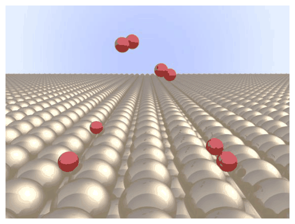
Hydrogen is expected to be a future energy source that does not depend on fossil fuels. Here, we will consider the hydrogen-storage process in a metal, which is related to hydrogen-transport and -storage technology.
PART A
As hydrogen is absorbed into the bulk of a metal via its surface, let us first consider the adsorption process of hydrogen at the metal surface, \(\ce{H2(g) -> 2H(ad)}\), where the gaseous and adsorbed states of hydrogen are represented as (g) and (ad), respectively. Hydrogen molecules (\(\ce{H2}\)) that reach the metal surface (M) dissociate at the surface and are adsorbed as \(\ce{H}\) atoms (Fig. 1). Here, the potential energy of \(\ce{H2}\) is represented by two variables: the interatomic distance, \(d\), and the height relative to the surface metal atom, \(z\). It is assumed that the axis along the two \(\ce{H}\) atoms is parallel to the surface and that the center of gravity is always on the vertical dotted line in Fig. 1. Fig. 2 shows the potential energy contour plot for the dissociation at the surface. The numerical values represent the potential energy in units of kJ per mole of \(\ce{H2}\). The solid line spacing is \(20\ \mathrm{kJ\,mol^{-1}}\), the dashed line spacing is \(100\ \mathrm{kJ\,mol^{-1}}\), and the spacing between solid and dashed lines is \(80\ \mathrm{kJ\,mol^{-1}}\). The zero-point vibration energy is ignored.
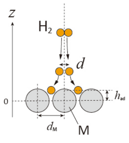
Fig.1 Definition of variables. Drawing is not in scale.
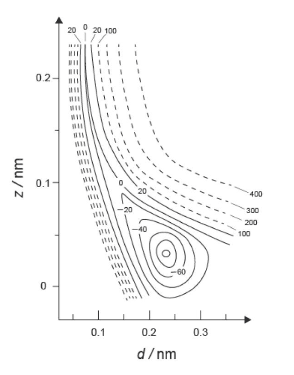
Fig.2
1.1 For each of the following items (i)–(iii), select the closest value from A–G.
(i) The interatomic distance for a gaseous \(\ce{H2}\) molecule
(ii) The interatomic distance between metal atoms (\(d_{\mathrm M}\) in Fig. 1)
(iii) The distance of adsorbed \(\ce{H}\) atoms from the surface (\(h_{\mathrm{AD}}\) in Fig. 1)
| A. \(0.03\ \mathrm{nm}\) | B. \(0.07\ \mathrm{nm}\) | C. \(0.11\ \mathrm{nm}\) | D. \(0.15\ \mathrm{nm}\) |
|---|---|---|---|
| E. \(0.19\ \mathrm{nm}\) | F. \(0.23\ \mathrm{nm}\) | G. \(0.27\ \mathrm{nm}\) |
1.2 For each of the following items (i)–(ii), select the closest value from A–H.
(i) the energy required for the dissociation of gaseous \(\ce{H2}\) to gaseous \(\ce{H}\) [\(\ce{H2(g) -> 2H(g)}\)]
(ii) the energy released during the adsorption of a gaseous \(\ce{H2}\) [\(\ce{H2(g) -> 2H(ad)}\)]
| A. \(20\ \mathrm{kJ\,mol^{-1}}\) | B. \(40\ \mathrm{kJ\,mol^{-1}}\) | C. \(60\ \mathrm{kJ\,mol^{-1}}\) | D. \(100\ \mathrm{kJ\,mol^{-1}}\) |
|---|---|---|---|
| E. \(150\ \mathrm{kJ\,mol^{-1}}\) | F. \(200\ \mathrm{kJ\,mol^{-1}}\) | G. \(300\ \mathrm{kJ\,mol^{-1}}\) | H. \(400\ \mathrm{kJ\,mol^{-1}}\) |
PART B
The adsorbed hydrogen atoms are then either absorbed into the bulk, or recombine and desorb back into the gas phase, as shown in the reactions (1a) and (1b). \(\ce{H(ab)}\) represents a hydrogen atom absorbed in the bulk.


The reaction rates per surface site for adsorption, desorption, and absorption are \(r_1[\mathrm{s^{-1}}]\), \(r_2[\mathrm{s^{-1}}]\) and \(r_3[\mathrm{s^{-1}}]\), respectively. They are expressed as:
\[ r_1=k_1P_{\ce{H2}}(1-\theta)^2 \tag{2} \]
\[ r_2=k_2\theta^2 \tag{3} \]
\[ r_3=k_3\theta \tag{4} \]
where \(k_1\ [\mathrm{s^{-1}\,Pa^{-1}}]\), \(k_2\ [\mathrm{s^{-1}}]\) and \(k_3\ [\mathrm{s^{-1}}]\) are the reaction rate constants and \(P_{\ce{H2}}\) is the pressure of \(\ce{H2}\). Among the sites available on the surface, \(\theta\) (\(0\leq\theta\leq1\)) is the fraction occupied by \(\ce{H}\) atoms. It is assumed that adsorption and desorption are fast compared to absorption (\(r_1,r_2\gg r_3\)) and that \(\theta\) remains constant.
1.3 \(r_3\) can be expressed as:
\[ r_3=\frac{k_3}{1+\sqrt{\dfrac{1}{P_{\ce{H2}}C}}} \tag{5} \]
Express \(C\) using \(k_1\) and \(k_2\).
A metal sample with a surface area of \(S=1.0\times10^{-3}\ \mathrm{m^2}\) was placed in a container (\(1\mathrm{L}=1.0\times10^{-3}\ \mathrm{m^3}\)) with \(\ce{H2}\) (\(P_{\ce{H2}}=1.0\times10^2\ \mathrm{Pa}\)). The density of hydrogen-atom adsorption sites on the surface was \(N=1.3\times10^{18}\ \mathrm{m^{-2}}\). The surface temperature was kept at \(T=400\ \mathrm K\). As the reaction (1) proceeded, \(P_{\ce{H2}}\) decreased at a constant rate of \(v=4.0\times10^{-4}\ \mathrm{Pa\,s^{-1}}\). Assume that \(\ce{H2}\) is an ideal gas and that the volume of the metal sample is negligible.
1.4 Calculate the amount of \(\ce{H}\) atoms in moles absorbed per unit area of the surface per unit time, \(A\ [\mathrm{mol\,s^{-1}\,m^{-2}}]\).
1.5 At \(T=400\ \mathrm K\), \(C\) equals \(1.0\times10^2\ \mathrm{Pa^{-1}}\). Calculate the value of \(k_3\) at \(400\ \mathrm K\). If you did not obtain the answer to 1.4, use \(A=3.6\times10^{-7}\ \mathrm{mol\,s^{-1}\,m^{-2}}\).
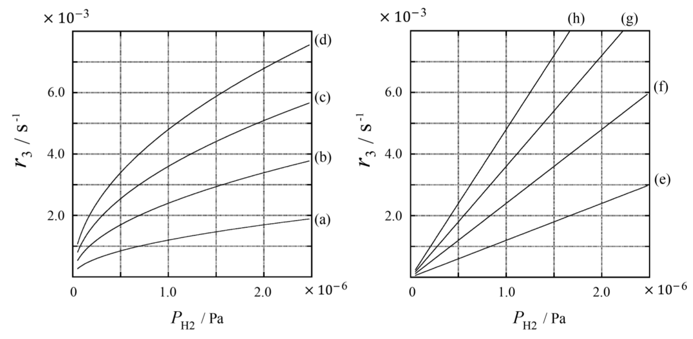
1.6 At a different \(T\), \(C=2.5\times10^3\ \mathrm{Pa^{-1}}\) and \(k_3=4.8\times10^{-2}\ \mathrm{s^{-1}}\) are given. For \(r_3\) as a function of \(P_{\ce{H2}}\) at this temperature, select the correct plot from (a)–(h).
Official English text of the problem.
Answers
- 1.1(i): B — \(0.07\ \mathrm{nm}\).
- 1.1(ii): F — \(0.23\ \mathrm{nm}\).
- 1.1(iii): A — \(0.03\ \mathrm{nm}\).
- 1.2(i): H — \(400\ \mathrm{kJ\,mol^{-1}}\) required.
- 1.2(ii): D — \(100\ \mathrm{kJ\,mol^{-1}}\) released.
- 1.3: \(\displaystyle C=\frac{k_1}{k_2}\).
- 1.4: \(\displaystyle A=2.4\times10^{-7}\ \mathrm{mol\,s^{-1}\,m^{-2}}\).
- 1.5: \(\displaystyle k_3=1.1\times10^{-1}\ \mathrm{s^{-1}}\).
- 1.6: Plot (b).
Solution
Hydrogen gas is dihydrogen, \(\ce{H2}\), SMILES [H][H]. Atomic hydrogen, \(\ce{H}\), has SMILES [H]. The labels (ad) and (ab) specify hydrogen at the surface and within the bulk, respectively; SMILES does not encode these environments or the metal–hydrogen coordination.
1.1
(i) Far from the surface, at large \(z\), the minimum-energy molecular configuration occurs at approximately
\[ d=0.07\ \mathrm{nm}. \]
This is the equilibrium bond length of gaseous dihydrogen. The answer is B.
(ii) The minimum corresponding to the adsorbed state is located at approximately
\[ (d,z)=(0.23,\ 0.03)\ \mathrm{nm}. \]
In Fig. 1, the two adsorbed hydrogen atoms occupy equivalent positions on opposite sides of the central metal atom. Their horizontal coordinates relative to that atom are \(-d_{\mathrm M}/2\) and \(+d_{\mathrm M}/2\), so their separation equals \(d_{\mathrm M}\). Thus,
\[ d_{\mathrm M}=d_{\text{adsorbed}}\approx0.23\ \mathrm{nm}, \]
giving F.
(iii) The vertical coordinate of the same minimum gives the adsorption height:
\[ h_{\mathrm{AD}}=z_{\min}\approx0.03\ \mathrm{nm}. \]
The answer is A.
1.2
The energy reference is the minimum for the gaseous molecule, approximately \(0\ \mathrm{kJ\,mol^{-1}}\). All energies in Fig. 2 are per mole of \(\ce{H2}\).
(i) For dissociation,
\[ \ce{H2(g) -> 2H(g)}, \]
both atoms must be far from the surface and far from each other: large \(z\) and large \(d\). The high-energy contours indicate a dissociation energy closest to
\[ \boxed{400\ \mathrm{kJ\,mol^{-1}}}. \]
The answer is H.
(ii) For dissociative adsorption,
\[ \ce{H2(g) -> 2H(ad)}, \]
the final state is the minimum near \((0.23,0.03)\ \mathrm{nm}\). Following the solid contours in \(20\ \mathrm{kJ\,mol^{-1}}\) increments places this minimum at approximately \(-100\ \mathrm{kJ\,mol^{-1}}\). Consequently,
\[ \Delta E_{\text{ads}}\approx-100\ \mathrm{kJ\,mol^{-1}}, \]
and the positive amount of energy released is
\[ \boxed{100\ \mathrm{kJ\,mol^{-1}}}. \]
The answer is D.
1.3
The reactions are
\[ \ce{H2(g) <=> 2H(ad)} \]
and
\[ \ce{H(ad) -> H(ab)}. \]
Each adsorption event creates two adsorbed atoms, each desorption event removes two, and each absorption event removes one. Constant coverage therefore requires
\[ \frac{d\theta}{dt}=2r_1-2r_2-r_3=0. \]
Because \(r_1,r_2\gg r_3\), adsorption and desorption are in approximate equilibrium:
\[ k_1P_{\ce{H2}}(1-\theta)^2\simeq k_2\theta^2. \]
Taking the nonnegative square root gives
\[ \frac{\theta}{1-\theta} =\sqrt{\frac{k_1P_{\ce{H2}}}{k_2}}. \]
Within this approximation,
\[ \theta =\frac{1}{1+\sqrt{\dfrac{k_2}{k_1P_{\ce{H2}}}}}, \]
so
\[ r_3=k_3\theta =\frac{k_3}{1+\sqrt{\dfrac{k_2}{k_1P_{\ce{H2}}}}}. \]
Comparison with equation (5) yields
\[ \boxed{C=\frac{k_1}{k_2}}. \]
Its units are \(\mathrm{Pa^{-1}}\), making \(P_{\ce{H2}}C\) dimensionless.
1.4
Use the ideal-gas equation with \(R=8.314\ \mathrm{Pa\,m^3\,mol^{-1}\,K^{-1}}\):
\[ n_{\ce{H2}}=\frac{P_{\ce{H2}}V}{RT}. \]
At constant volume and temperature, the rate of disappearance of gaseous dihydrogen is
\[ -\frac{dn_{\ce{H2}}}{dt} =\frac{Vv}{RT} =\frac{ (1.0\times10^{-3}\ \mathrm{m^3}) (4.0\times10^{-4}\ \mathrm{Pa\,s^{-1}}) }{ (8.314\ \mathrm{Pa\,m^3\,mol^{-1}\,K^{-1}}) (400\ \mathrm K) } =1.20\times10^{-10}\ \mathrm{mol\,s^{-1}}. \]
Since the surface coverage remains constant, hydrogen does not accumulate on the surface. The net process is therefore
\[ \ce{H2(g) -> 2H(ab)}. \]
Two moles of hydrogen atoms enter the bulk for each mole of gas consumed. Dividing by the surface area,
\[ A=\frac{2Vv}{RTS} =\frac{2(1.20\times10^{-10}\ \mathrm{mol\,s^{-1}})} {1.0\times10^{-3}\ \mathrm{m^2}}. \]
Thus,
\[ \boxed{A=2.4\times10^{-7}\ \mathrm{mol\,s^{-1}\,m^{-2}}}. \]
1.5
At the stated pressure,
\[ P_{\ce{H2}}C =(1.0\times10^2\ \mathrm{Pa}) (1.0\times10^2\ \mathrm{Pa^{-1}}) =1.0\times10^4. \]
Hence,
\[ \theta=\frac{1}{1+(P_{\ce{H2}}C)^{-1/2}} =\frac{1}{1+0.010} =0.9901. \]
Each absorption event transfers one hydrogen atom. Using \(N_{\mathrm A}=6.022\times10^{23}\ \mathrm{mol^{-1}}\), the molar absorption rate and the rate per surface site satisfy
\[ A=\frac{Nr_3}{N_{\mathrm A}} =\frac{Nk_3\theta}{N_{\mathrm A}}. \]
Therefore, using the unrounded result from 1.4,
\[ k_3=\frac{AN_{\mathrm A}}{N\theta} =\frac{ (2.405\times10^{-7}\ \mathrm{mol\,s^{-1}\,m^{-2}}) (6.022\times10^{23}\ \mathrm{mol^{-1}}) }{ (1.3\times10^{18}\ \mathrm{m^{-2}})(0.9901) } =0.1125\ \mathrm{s^{-1}}. \]
To two significant figures,
\[ \boxed{k_3=1.1\times10^{-1}\ \mathrm{s^{-1}}}. \]
1.6
Rewrite equation (5) as
\[ r_3=k_3\frac{\sqrt{CP_{\ce{H2}}}} {1+\sqrt{CP_{\ce{H2}}}}. \]
Over the plotted pressure range,
\[ CP_{\ce{H2}} \leq (2.5\times10^3\ \mathrm{Pa^{-1}}) (2.5\times10^{-6}\ \mathrm{Pa}) =6.25\times10^{-3}\ll1. \]
Thus, approximately,
\[ r_3\simeq k_3\sqrt{CP_{\ce{H2}}}. \]
The curve starts at the origin, rises with increasing pressure, and bends downward. This selects the family (a)–(d).
To identify its magnitude, take \(P_{\ce{H2}}=1.0\times10^{-6}\ \mathrm{Pa}\). Then
\[ \sqrt{CP_{\ce{H2}}} =\sqrt{(2.5\times10^3)(1.0\times10^{-6})} =0.050, \]
and the full expression gives
\[ r_3=(4.8\times10^{-2}) \frac{0.050}{1.050} =2.29\times10^{-3}\ \mathrm{s^{-1}}. \]
The low-pressure approximation gives \(2.4\times10^{-3}\ \mathrm{s^{-1}}\), matching the scale of curve (b). Thus,
\[ \boxed{\text{Plot (b)}}. \]
The solution was checked against the official solution.
IChO 2021 · Theorieaufgabe 1
Wasserstoff an einer Metalloberfläche
Wasserstoff gilt als zukünftiger Energieträger, der nicht von fossilen Brennstoffen abhängt. Hier betrachten wir den Prozess der Wasserstoffspeicherung in einem Metall, der mit Technologien zum Transport und zur Speicherung von Wasserstoff zusammenhängt.
TEIL A
Da Wasserstoff über die Oberfläche eines Metalls in dessen Inneres aufgenommen wird, betrachten wir zunächst den Adsorptionsprozess von Wasserstoff an der Metalloberfläche, \(\ce{H2(g) -> 2H(ad)}\), wobei der gasförmige und der adsorbierte Zustand des Wasserstoffs mit (g) bzw. (ad) bezeichnet werden. Wasserstoffmoleküle (\(\ce{H2}\)), die die Metalloberfläche (M) erreichen, dissoziieren an der Oberfläche und werden als \(\ce{H}\)-Atome adsorbiert (Abb. 1). Die potenzielle Energie von \(\ce{H2}\) wird hier durch zwei Variablen beschrieben: den Abstand zwischen den Atomen, \(d\), und die Höhe relativ zum Metallatom an der Oberfläche, \(z\). Es wird angenommen, dass die Achse durch die beiden \(\ce{H}\)-Atome parallel zur Oberfläche verläuft und sich der Schwerpunkt stets auf der vertikalen gepunkteten Linie in Abb. 1 befindet. Abb. 2 zeigt das Konturdiagramm der potenziellen Energie für die Dissoziation an der Oberfläche. Die Zahlenwerte geben die potenzielle Energie in kJ pro Mol \(\ce{H2}\) an. Der Abstand zwischen den durchgezogenen Linien beträgt \(20\ \mathrm{kJ\,mol^{-1}}\), der Abstand zwischen den gestrichelten Linien \(100\ \mathrm{kJ\,mol^{-1}}\) und der Abstand zwischen durchgezogenen und gestrichelten Linien \(80\ \mathrm{kJ\,mol^{-1}}\). Die Nullpunktsschwingungsenergie wird vernachlässigt.
Abb. 1 Definition der Variablen. Die Zeichnung ist nicht maßstabsgetreu.
Abb. 2
1.1 Wählen Sie für jede der folgenden Größen (i)–(iii) den nächstliegenden Wert aus A–G aus.
(i) Der Abstand zwischen den Atomen eines gasförmigen \(\ce{H2}\)-Moleküls
(ii) Der Abstand zwischen den Metallatomen (\(d_{\mathrm M}\) in Abb. 1)
(iii) Der Abstand der adsorbierten \(\ce{H}\)-Atome von der Oberfläche (\(h_{\mathrm{AD}}\) in Abb. 1)
| A. \(0.03\ \mathrm{nm}\) | B. \(0.07\ \mathrm{nm}\) | C. \(0.11\ \mathrm{nm}\) | D. \(0.15\ \mathrm{nm}\) |
|---|---|---|---|
| E. \(0.19\ \mathrm{nm}\) | F. \(0.23\ \mathrm{nm}\) | G. \(0.27\ \mathrm{nm}\) |
1.2 Wählen Sie für jede der folgenden Größen (i)–(ii) den nächstliegenden Wert aus A–H aus.
(i) die für die Dissoziation von gasförmigem \(\ce{H2}\) zu gasförmigem \(\ce{H}\) erforderliche Energie [\(\ce{H2(g) -> 2H(g)}\)]
(ii) die bei der Adsorption von gasförmigem \(\ce{H2}\) freigesetzte Energie [\(\ce{H2(g) -> 2H(ad)}\)]
| A. \(20\ \mathrm{kJ\,mol^{-1}}\) | B. \(40\ \mathrm{kJ\,mol^{-1}}\) | C. \(60\ \mathrm{kJ\,mol^{-1}}\) | D. \(100\ \mathrm{kJ\,mol^{-1}}\) |
|---|---|---|---|
| E. \(150\ \mathrm{kJ\,mol^{-1}}\) | F. \(200\ \mathrm{kJ\,mol^{-1}}\) | G. \(300\ \mathrm{kJ\,mol^{-1}}\) | H. \(400\ \mathrm{kJ\,mol^{-1}}\) |
TEIL B
Die adsorbierten Wasserstoffatome werden anschließend entweder in das Metallinnere aufgenommen oder rekombinieren und desorbieren zurück in die Gasphase, wie in den Reaktionen (1a) und (1b) dargestellt. \(\ce{H(ab)}\) bezeichnet ein im Metallinneren absorbiertes Wasserstoffatom.
Die Reaktionsgeschwindigkeiten pro Oberflächenplatz für Adsorption, Desorption und Absorption sind \(r_1[\mathrm{s^{-1}}]\), \(r_2[\mathrm{s^{-1}}]\) bzw. \(r_3[\mathrm{s^{-1}}]\). Sie werden wie folgt ausgedrückt:
\[ r_1=k_1P_{\ce{H2}}(1-\theta)^2 \tag{2} \]
\[ r_2=k_2\theta^2 \tag{3} \]
\[ r_3=k_3\theta \tag{4} \]
wobei \(k_1\ [\mathrm{s^{-1}\,Pa^{-1}}]\), \(k_2\ [\mathrm{s^{-1}}]\) und \(k_3\ [\mathrm{s^{-1}}]\) die Reaktionsgeschwindigkeitskonstanten sind und \(P_{\ce{H2}}\) der Druck von \(\ce{H2}\) ist. Von den auf der Oberfläche verfügbaren Plätzen ist \(\theta\) (\(0\leq\theta\leq1\)) der Anteil, der von \(\ce{H}\)-Atomen besetzt ist. Es wird angenommen, dass Adsorption und Desorption im Vergleich zur Absorption schnell sind (\(r_1,r_2\gg r_3\)) und dass \(\theta\) konstant bleibt.
1.3 \(r_3\) lässt sich wie folgt ausdrücken:
\[ r_3=\frac{k_3}{1+\sqrt{\dfrac{1}{P_{\ce{H2}}C}}} \tag{5} \]
Drücken Sie \(C\) durch \(k_1\) und \(k_2\) aus.
Eine Metallprobe mit einer Oberfläche von \(S=1.0\times10^{-3}\ \mathrm{m^2}\) wurde in einen Behälter (\(1\mathrm{L}=1.0\times10^{-3}\ \mathrm{m^3}\)) mit \(\ce{H2}\) (\(P_{\ce{H2}}=1.0\times10^2\ \mathrm{Pa}\)) eingebracht. Die Dichte der Adsorptionsplätze für Wasserstoffatome auf der Oberfläche betrug \(N=1.3\times10^{18}\ \mathrm{m^{-2}}\). Die Oberflächentemperatur wurde bei \(T=400\ \mathrm K\) konstant gehalten. Während Reaktion (1) ablief, nahm \(P_{\ce{H2}}\) mit einer konstanten Geschwindigkeit von \(v=4.0\times10^{-4}\ \mathrm{Pa\,s^{-1}}\) ab. Nehmen Sie an, dass \(\ce{H2}\) ein ideales Gas ist und das Volumen der Metallprobe vernachlässigbar ist.
1.4 Berechnen Sie die Stoffmenge der pro Flächeneinheit der Oberfläche und pro Zeiteinheit absorbierten \(\ce{H}\)-Atome in Mol, \(A\ [\mathrm{mol\,s^{-1}\,m^{-2}}]\).
1.5 Bei \(T=400\ \mathrm K\) beträgt \(C\) \(1.0\times10^2\ \mathrm{Pa^{-1}}\). Berechnen Sie den Wert von \(k_3\) bei \(400\ \mathrm K\). Falls Sie keine Antwort auf 1.4 erhalten haben, verwenden Sie \(A=3.6\times10^{-7}\ \mathrm{mol\,s^{-1}\,m^{-2}}\).
1.6 Bei einer anderen Temperatur \(T\) sind \(C=2.5\times10^3\ \mathrm{Pa^{-1}}\) und \(k_3=4.8\times10^{-2}\ \mathrm{s^{-1}}\) gegeben. Wählen Sie aus (a)–(h) den richtigen Graphen für \(r_3\) als Funktion von \(P_{\ce{H2}}\) bei dieser Temperatur aus.
Aufgabentext aus dem offiziellen englischen Text übersetzt.
Antworten
- 1.1(i): B — \(0.07\ \mathrm{nm}\).
- 1.1(ii): F — \(0.23\ \mathrm{nm}\).
- 1.1(iii): A — \(0.03\ \mathrm{nm}\).
- 1.2(i): H — \(400\ \mathrm{kJ\,mol^{-1}}\) erforderlich.
- 1.2(ii): D — \(100\ \mathrm{kJ\,mol^{-1}}\) freigesetzt.
- 1.3: \(\displaystyle C=\frac{k_1}{k_2}\).
- 1.4: \(\displaystyle A=2.4\times10^{-7}\ \mathrm{mol\,s^{-1}\,m^{-2}}\).
- 1.5: \(\displaystyle k_3=1.1\times10^{-1}\ \mathrm{s^{-1}}\).
- 1.6: Graph (b).
Lösung
Wasserstoffgas ist Diwasserstoff, \(\ce{H2}\), mit der SMILES-Schreibweise [H][H]. Atomarer Wasserstoff, \(\ce{H}\), hat die SMILES-Schreibweise [H]. Die Kennzeichnungen (ad) und (ab) bezeichnen Wasserstoff an der Oberfläche bzw. im Metallinneren; SMILES bildet diese Umgebungen oder die Metall–Wasserstoff-Koordination nicht ab.
1.1
(i) Weit von der Oberfläche entfernt, bei großem \(z\), liegt die Molekülkonfiguration mit der geringsten Energie ungefähr bei
\[ d=0.07\ \mathrm{nm}. \]
Dies ist die Gleichgewichtsbindungslänge von gasförmigem Diwasserstoff. Die Antwort ist B.
(ii) Das Minimum, das dem adsorbierten Zustand entspricht, liegt ungefähr bei
\[ (d,z)=(0.23,\ 0.03)\ \mathrm{nm}. \]
In Abb. 1 besetzen die beiden adsorbierten Wasserstoffatome äquivalente Positionen auf gegenüberliegenden Seiten des zentralen Metallatoms. Ihre horizontalen Koordinaten relativ zu diesem Atom sind \(-d_{\mathrm M}/2\) und \(+d_{\mathrm M}/2\), sodass ihr Abstand gleich \(d_{\mathrm M}\) ist. Somit gilt
\[ d_{\mathrm M}=d_{\text{adsorbiert}}\approx0.23\ \mathrm{nm}, \]
woraus sich F ergibt.
(iii) Die vertikale Koordinate desselben Minimums liefert die Adsorptionshöhe:
\[ h_{\mathrm{AD}}=z_{\min}\approx0.03\ \mathrm{nm}. \]
Die Antwort ist A.
1.2
Als Energiebezug dient das Minimum für das gasförmige Molekül bei ungefähr \(0\ \mathrm{kJ\,mol^{-1}}\). Alle Energien in Abb. 2 beziehen sich auf ein Mol \(\ce{H2}\).
(i) Bei der Dissoziation
\[ \ce{H2(g) -> 2H(g)}, \]
müssen beide Atome sowohl weit von der Oberfläche als auch weit voneinander entfernt sein: großes \(z\) und großes \(d\). Die durch die Konturlinien hoher Energie angezeigte Dissoziationsenergie liegt am nächsten am Wert
\[ \boxed{400\ \mathrm{kJ\,mol^{-1}}}. \]
Die Antwort ist H.
(ii) Bei der dissoziativen Adsorption
\[ \ce{H2(g) -> 2H(ad)}, \]
ist der Endzustand das Minimum nahe \((0.23,0.03)\ \mathrm{nm}\). Folgt man den durchgezogenen Konturlinien in Schritten von \(20\ \mathrm{kJ\,mol^{-1}}\), so liegt dieses Minimum bei ungefähr \(-100\ \mathrm{kJ\,mol^{-1}}\). Folglich gilt
\[ \Delta E_{\text{ads}}\approx-100\ \mathrm{kJ\,mol^{-1}}, \]
und der positive Betrag der freigesetzten Energie ist
\[ \boxed{100\ \mathrm{kJ\,mol^{-1}}}. \]
Die Antwort ist D.
1.3
Die Reaktionen lauten
\[ \ce{H2(g) <=> 2H(ad)} \]
und
\[ \ce{H(ad) -> H(ab)}. \]
Jeder Adsorptionsvorgang erzeugt zwei adsorbierte Atome, jeder Desorptionsvorgang entfernt zwei und jeder Absorptionsvorgang entfernt eines. Ein konstanter Bedeckungsgrad erfordert daher
\[ \frac{d\theta}{dt}=2r_1-2r_2-r_3=0. \]
Da \(r_1,r_2\gg r_3\), befinden sich Adsorption und Desorption näherungsweise im Gleichgewicht:
\[ k_1P_{\ce{H2}}(1-\theta)^2\simeq k_2\theta^2. \]
Das Ziehen der nichtnegativen Quadratwurzel ergibt
\[ \frac{\theta}{1-\theta} =\sqrt{\frac{k_1P_{\ce{H2}}}{k_2}}. \]
Im Rahmen dieser Näherung gilt
\[ \theta =\frac{1}{1+\sqrt{\dfrac{k_2}{k_1P_{\ce{H2}}}}}, \]
sodass
\[ r_3=k_3\theta =\frac{k_3}{1+\sqrt{\dfrac{k_2}{k_1P_{\ce{H2}}}}}. \]
Der Vergleich mit Gleichung (5) liefert
\[ \boxed{C=\frac{k_1}{k_2}}. \]
Die Einheit ist \(\mathrm{Pa^{-1}}\), wodurch \(P_{\ce{H2}}C\) dimensionslos ist.
1.4
Wir verwenden die ideale Gasgleichung mit \(R=8.314\ \mathrm{Pa\,m^3\,mol^{-1}\,K^{-1}}\):
\[ n_{\ce{H2}}=\frac{P_{\ce{H2}}V}{RT}. \]
Bei konstantem Volumen und konstanter Temperatur beträgt die Geschwindigkeit der Abnahme der Stoffmenge des gasförmigen Diwasserstoffs
\[ -\frac{dn_{\ce{H2}}}{dt} =\frac{Vv}{RT} =\frac{ (1.0\times10^{-3}\ \mathrm{m^3}) (4.0\times10^{-4}\ \mathrm{Pa\,s^{-1}}) }{ (8.314\ \mathrm{Pa\,m^3\,mol^{-1}\,K^{-1}}) (400\ \mathrm K) } =1.20\times10^{-10}\ \mathrm{mol\,s^{-1}}. \]
Da der Bedeckungsgrad der Oberfläche konstant bleibt, reichert sich auf der Oberfläche kein Wasserstoff an. Der Nettoprozess lautet daher
\[ \ce{H2(g) -> 2H(ab)}. \]
Für jedes verbrauchte Mol Gas gelangen zwei Mol Wasserstoffatome in das Metallinnere. Durch Division durch die Oberfläche ergibt sich
\[ A=\frac{2Vv}{RTS} =\frac{2(1.20\times10^{-10}\ \mathrm{mol\,s^{-1}})} {1.0\times10^{-3}\ \mathrm{m^2}}. \]
Somit gilt
\[ \boxed{A=2.4\times10^{-7}\ \mathrm{mol\,s^{-1}\,m^{-2}}}. \]
1.5
Bei dem angegebenen Druck gilt
\[ P_{\ce{H2}}C =(1.0\times10^2\ \mathrm{Pa}) (1.0\times10^2\ \mathrm{Pa^{-1}}) =1.0\times10^4. \]
Daraus folgt
\[ \theta=\frac{1}{1+(P_{\ce{H2}}C)^{-1/2}} =\frac{1}{1+0.010} =0.9901. \]
Bei jedem Absorptionsvorgang wird ein Wasserstoffatom übertragen. Mit \(N_{\mathrm A}=6.022\times10^{23}\ \mathrm{mol^{-1}}\) gilt für die molare Absorptionsgeschwindigkeit und die Geschwindigkeit pro Oberflächenplatz
\[ A=\frac{Nr_3}{N_{\mathrm A}} =\frac{Nk_3\theta}{N_{\mathrm A}}. \]
Unter Verwendung des ungerundeten Ergebnisses aus 1.4 folgt daher
\[ k_3=\frac{AN_{\mathrm A}}{N\theta} =\frac{ (2.405\times10^{-7}\ \mathrm{mol\,s^{-1}\,m^{-2}}) (6.022\times10^{23}\ \mathrm{mol^{-1}}) }{ (1.3\times10^{18}\ \mathrm{m^{-2}})(0.9901) } =0.1125\ \mathrm{s^{-1}}. \]
Auf zwei signifikante Stellen gerundet ergibt sich
\[ \boxed{k_3=1.1\times10^{-1}\ \mathrm{s^{-1}}}. \]
1.6
Wir schreiben Gleichung (5) um zu
\[ r_3=k_3\frac{\sqrt{CP_{\ce{H2}}}} {1+\sqrt{CP_{\ce{H2}}}}. \]
Im dargestellten Druckbereich gilt
\[ CP_{\ce{H2}} \leq (2.5\times10^3\ \mathrm{Pa^{-1}}) (2.5\times10^{-6}\ \mathrm{Pa}) =6.25\times10^{-3}\ll1. \]
Somit gilt näherungsweise
\[ r_3\simeq k_3\sqrt{CP_{\ce{H2}}}. \]
Die Kurve beginnt im Ursprung, steigt mit zunehmendem Druck an und ist nach unten gekrümmt. Damit kommt die Gruppe (a)–(d) infrage.
Um die Größenordnung zu bestimmen, setzen wir \(P_{\ce{H2}}=1.0\times10^{-6}\ \mathrm{Pa}\). Dann gilt
\[ \sqrt{CP_{\ce{H2}}} =\sqrt{(2.5\times10^3)(1.0\times10^{-6})} =0.050, \]
und der vollständige Ausdruck liefert
\[ r_3=(4.8\times10^{-2}) \frac{0.050}{1.050} =2.29\times10^{-3}\ \mathrm{s^{-1}}. \]
Die Näherung für niedrige Drücke ergibt \(2.4\times10^{-3}\ \mathrm{s^{-1}}\), was mit der Größenordnung von Kurve (b) übereinstimmt. Somit gilt
\[ \boxed{\text{Graph (b)}}. \]
Die Lösung wurde mit der offiziellen Lösung abgeglichen.
IChO 2021 · Teori sorusu 1
Metal Yüzeyinde Hidrojen
Hidrojenin gelecekte fosil yakıtlara bağımlı olmayan bir enerji kaynağı olması beklenmektedir. Burada, hidrojen taşıma ve depolama teknolojisiyle ilişkili olan, bir metalde hidrojen depolama sürecini ele alacağız.
BÖLÜM A
Hidrojen, metalin yüzeyi üzerinden metalin iç hacmine absorplandığından, önce hidrojenin metal yüzeyindeki adsorpsiyon sürecini, \(\ce{H2(g) -> 2H(ad)}\), ele alalım; burada hidrojenin gaz ve adsorplanmış hâlleri sırasıyla (g) ve (ad) ile gösterilmektedir. Metal yüzeyine (M) ulaşan hidrojen molekülleri (\(\ce{H2}\)) yüzeyde ayrışır ve \(\ce{H}\) atomları olarak adsorplanır (Şekil 1). Burada \(\ce{H2}\)'nin potansiyel enerjisi iki değişkenle ifade edilmektedir: atomlar arası uzaklık, \(d\), ve yüzeydeki metal atomuna göre yükseklik, \(z\). İki \(\ce{H}\) atomundan geçen eksenin yüzeye paralel olduğu ve ağırlık merkezinin her zaman Şekil 1'deki düşey noktalı çizgi üzerinde bulunduğu varsayılmaktadır. Şekil 2, yüzeydeki ayrışmaya ait potansiyel enerji eş yükselti eğrilerini göstermektedir. Sayısal değerler, potansiyel enerjiyi bir mol \(\ce{H2}\) başına kJ biriminde ifade etmektedir. Sürekli çizgiler arasındaki enerji farkı \(20\ \mathrm{kJ\,mol^{-1}}\), kesikli çizgiler arasındaki enerji farkı \(100\ \mathrm{kJ\,mol^{-1}}\), sürekli ve kesikli çizgiler arasındaki enerji farkı ise \(80\ \mathrm{kJ\,mol^{-1}}\)'dir. Sıfır noktası titreşim enerjisi ihmal edilmektedir.
Şekil 1 Değişkenlerin tanımı. Çizim ölçekli değildir.
Şekil 2
1.1 Aşağıdaki (i)–(iii) maddelerinin her biri için A–G seçenekleri arasından en yakın değeri seçiniz.
(i) Gaz hâlindeki bir \(\ce{H2}\) molekülünde atomlar arası uzaklık
(ii) Metal atomları arasındaki uzaklık (Şekil 1'deki \(d_{\mathrm M}\))
(iii) Adsorplanmış \(\ce{H}\) atomlarının yüzeyden uzaklığı (Şekil 1'deki \(h_{\mathrm{AD}}\))
| A. \(0.03\ \mathrm{nm}\) | B. \(0.07\ \mathrm{nm}\) | C. \(0.11\ \mathrm{nm}\) | D. \(0.15\ \mathrm{nm}\) |
|---|---|---|---|
| E. \(0.19\ \mathrm{nm}\) | F. \(0.23\ \mathrm{nm}\) | G. \(0.27\ \mathrm{nm}\) |
1.2 Aşağıdaki (i)–(ii) maddelerinin her biri için A–H seçenekleri arasından en yakın değeri seçiniz.
(i) gaz hâlindeki \(\ce{H2}\)'nin gaz hâlindeki \(\ce{H}\)'ye ayrışması için gereken enerji [\(\ce{H2(g) -> 2H(g)}\)]
(ii) gaz hâlindeki bir \(\ce{H2}\)'nin adsorpsiyonu sırasında açığa çıkan enerji [\(\ce{H2(g) -> 2H(ad)}\)]
| A. \(20\ \mathrm{kJ\,mol^{-1}}\) | B. \(40\ \mathrm{kJ\,mol^{-1}}\) | C. \(60\ \mathrm{kJ\,mol^{-1}}\) | D. \(100\ \mathrm{kJ\,mol^{-1}}\) |
|---|---|---|---|
| E. \(150\ \mathrm{kJ\,mol^{-1}}\) | F. \(200\ \mathrm{kJ\,mol^{-1}}\) | G. \(300\ \mathrm{kJ\,mol^{-1}}\) | H. \(400\ \mathrm{kJ\,mol^{-1}}\) |
BÖLÜM B
Adsorplanmış hidrojen atomları daha sonra, (1a) ve (1b) tepkimelerinde gösterildiği gibi, ya metalin iç hacmine absorplanır ya da yeniden birleşip desorplanarak gaz fazına geri döner. \(\ce{H(ab)}\), metalin iç hacmine absorplanmış bir hidrojen atomunu temsil etmektedir.
Adsorpsiyon, desorpsiyon ve absorpsiyon için yüzey merkezi başına tepkime hızları sırasıyla \(r_1[\mathrm{s^{-1}}]\), \(r_2[\mathrm{s^{-1}}]\) ve \(r_3[\mathrm{s^{-1}}]\)'tür. Bu hızlar aşağıdaki gibi ifade edilir:
\[ r_1=k_1P_{\ce{H2}}(1-\theta)^2 \tag{2} \]
\[ r_2=k_2\theta^2 \tag{3} \]
\[ r_3=k_3\theta \tag{4} \]
Burada \(k_1\ [\mathrm{s^{-1}\,Pa^{-1}}]\), \(k_2\ [\mathrm{s^{-1}}]\) ve \(k_3\ [\mathrm{s^{-1}}]\) tepkime hız sabitleri, \(P_{\ce{H2}}\) ise \(\ce{H2}\)'nin basıncıdır. \(\theta\) (\(0\leq\theta\leq1\)), yüzeydeki kullanılabilir merkezlerin \(\ce{H}\) atomları tarafından işgal edilen kesridir. Adsorpsiyon ve desorpsiyonun absorpsiyona kıyasla hızlı olduğu (\(r_1,r_2\gg r_3\)) ve \(\theta\)'nın sabit kaldığı varsayılmaktadır.
1.3 \(r_3\) aşağıdaki gibi ifade edilebilir:
\[ r_3=\frac{k_3}{1+\sqrt{\dfrac{1}{P_{\ce{H2}}C}}} \tag{5} \]
\(C\)'yi \(k_1\) ve \(k_2\) cinsinden ifade ediniz.
Yüzey alanı \(S=1.0\times10^{-3}\ \mathrm{m^2}\) olan bir metal numunesi, \(\ce{H2}\) (\(P_{\ce{H2}}=1.0\times10^2\ \mathrm{Pa}\)) içeren bir kaba (\(1\mathrm{L}=1.0\times10^{-3}\ \mathrm{m^3}\)) yerleştirilmiştir. Yüzeydeki hidrojen atomu adsorpsiyon merkezlerinin yoğunluğu \(N=1.3\times10^{18}\ \mathrm{m^{-2}}\)'dir. Yüzey sıcaklığı \(T=400\ \mathrm K\)'de sabit tutulmuştur. Tepkime (1) ilerledikçe \(P_{\ce{H2}}\), sabit bir \(v=4.0\times10^{-4}\ \mathrm{Pa\,s^{-1}}\) hızıyla azalmıştır. \(\ce{H2}\)'nin ideal gaz olduğunu ve metal numunesinin hacminin ihmal edilebilir olduğunu varsayınız.
1.4 Birim yüzey alanı başına birim zamanda absorplanan \(\ce{H}\) atomlarının mol cinsinden miktarını, \(A\ [\mathrm{mol\,s^{-1}\,m^{-2}}]\), hesaplayınız.
1.5 \(T=400\ \mathrm K\)'de \(C\), \(1.0\times10^2\ \mathrm{Pa^{-1}}\)'e eşittir. \(400\ \mathrm K\)'deki \(k_3\) değerini hesaplayınız. 1.4'ün cevabını bulamadıysanız \(A=3.6\times10^{-7}\ \mathrm{mol\,s^{-1}\,m^{-2}}\) değerini kullanınız.
1.6 Farklı bir \(T\) için \(C=2.5\times10^3\ \mathrm{Pa^{-1}}\) ve \(k_3=4.8\times10^{-2}\ \mathrm{s^{-1}}\) değerleri verilmiştir. Bu sıcaklıkta \(P_{\ce{H2}}\)'nin fonksiyonu olarak \(r_3\)'ü gösteren doğru grafiği (a)–(h) arasından seçiniz.
Soru metni resmi İngilizce metinden çevrilmiştir.
Cevaplar
- 1.1(i): B — \(0.07\ \mathrm{nm}\).
- 1.1(ii): F — \(0.23\ \mathrm{nm}\).
- 1.1(iii): A — \(0.03\ \mathrm{nm}\).
- 1.2(i): H — \(400\ \mathrm{kJ\,mol^{-1}}\) gerekir.
- 1.2(ii): D — \(100\ \mathrm{kJ\,mol^{-1}}\) açığa çıkar.
- 1.3: \(\displaystyle C=\frac{k_1}{k_2}\).
- 1.4: \(\displaystyle A=2.4\times10^{-7}\ \mathrm{mol\,s^{-1}\,m^{-2}}\).
- 1.5: \(\displaystyle k_3=1.1\times10^{-1}\ \mathrm{s^{-1}}\).
- 1.6: Grafik (b).
Çözüm
Hidrojen gazı, SMILES gösterimi [H][H] olan dihidrojendir, \(\ce{H2}\). Atomik hidrojenin, \(\ce{H}\), SMILES gösterimi [H]'dir. (ad) ve (ab) etiketleri sırasıyla yüzeydeki ve metalin iç hacmindeki hidrojeni belirtir; SMILES bu ortamları veya metal–hidrojen koordinasyonunu kodlamaz.
1.1
(i) Yüzeyden uzakta, büyük \(z\) değerlerinde, minimum enerjili moleküler konfigürasyon yaklaşık olarak şu uzaklıkta görülür:
\[ d=0.07\ \mathrm{nm}. \]
Bu, gaz hâlindeki dihidrojenin denge bağ uzunluğudur. Cevap B'dir.
(ii) Adsorplanmış hâle karşılık gelen minimum yaklaşık olarak şu konumdadır:
\[ (d,z)=(0.23,\ 0.03)\ \mathrm{nm}. \]
Şekil 1'de, adsorplanmış iki hidrojen atomu merkezdeki metal atomunun karşılıklı iki yanında eşdeğer konumları işgal eder. Bu atoma göre yatay koordinatları \(-d_{\mathrm M}/2\) ve \(+d_{\mathrm M}/2\) olduğundan aralarındaki uzaklık \(d_{\mathrm M}\)'ye eşittir. Dolayısıyla,
\[ d_{\mathrm M}=d_{\text{adsorplanmış}}\approx0.23\ \mathrm{nm}, \]
olup cevap F'dir.
(iii) Aynı minimumun düşey koordinatı adsorpsiyon yüksekliğini verir:
\[ h_{\mathrm{AD}}=z_{\min}\approx0.03\ \mathrm{nm}. \]
Cevap A'dır.
1.2
Enerji referansı, gaz hâlindeki molekül için yaklaşık \(0\ \mathrm{kJ\,mol^{-1}}\) olan minimumdur. Şekil 2'deki tüm enerjiler bir mol \(\ce{H2}\) başınadır.
(i) Ayrışma için,
\[ \ce{H2(g) -> 2H(g)}, \]
her iki atomun da hem yüzeyden hem de birbirinden uzakta olması gerekir: \(z\) ve \(d\) büyük olmalıdır. Yüksek enerjili eş yükselti eğrileri, ayrışma enerjisinin en yakın olduğu değerin şu olduğunu gösterir:
\[ \boxed{400\ \mathrm{kJ\,mol^{-1}}}. \]
Cevap H'dir.
(ii) Ayrışmalı adsorpsiyon için,
\[ \ce{H2(g) -> 2H(ad)}, \]
son hâl, \((0.23,0.03)\ \mathrm{nm}\) yakınındaki minimumdur. Sürekli eş yükselti eğrileri \(20\ \mathrm{kJ\,mol^{-1}}\)'lük artışlarla izlendiğinde bu minimumun yaklaşık \(-100\ \mathrm{kJ\,mol^{-1}}\)'de olduğu bulunur. Buna göre,
\[ \Delta E_{\text{ads}}\approx-100\ \mathrm{kJ\,mol^{-1}}, \]
ve açığa çıkan enerjinin pozitif miktarı şöyledir:
\[ \boxed{100\ \mathrm{kJ\,mol^{-1}}}. \]
Cevap D'dir.
1.3
Tepkimeler şöyledir:
\[ \ce{H2(g) <=> 2H(ad)} \]
ve
\[ \ce{H(ad) -> H(ab)}. \]
Her adsorpsiyon olayı yüzeyde iki adsorplanmış atom oluşturur, her desorpsiyon olayı yüzeyden iki atom uzaklaştırır ve her absorpsiyon olayı yüzeyden bir atom uzaklaştırır. Bu nedenle yüzey örtülme oranının sabit olması şu koşulu gerektirir:
\[ \frac{d\theta}{dt}=2r_1-2r_2-r_3=0. \]
\(r_1,r_2\gg r_3\) olduğundan adsorpsiyon ve desorpsiyon yaklaşık olarak dengededir:
\[ k_1P_{\ce{H2}}(1-\theta)^2\simeq k_2\theta^2. \]
Negatif olmayan karekök alındığında şu elde edilir:
\[ \frac{\theta}{1-\theta} =\sqrt{\frac{k_1P_{\ce{H2}}}{k_2}}. \]
Bu yaklaşım kapsamında,
\[ \theta =\frac{1}{1+\sqrt{\dfrac{k_2}{k_1P_{\ce{H2}}}}}, \]
dolayısıyla
\[ r_3=k_3\theta =\frac{k_3}{1+\sqrt{\dfrac{k_2}{k_1P_{\ce{H2}}}}}. \]
Denklem (5) ile karşılaştırıldığında şu elde edilir:
\[ \boxed{C=\frac{k_1}{k_2}}. \]
Birimi \(\mathrm{Pa^{-1}}\) olduğundan \(P_{\ce{H2}}C\) boyutsuzdur.
1.4
\(R=8.314\ \mathrm{Pa\,m^3\,mol^{-1}\,K^{-1}}\) değeriyle ideal gaz denklemini kullanalım:
\[ n_{\ce{H2}}=\frac{P_{\ce{H2}}V}{RT}. \]
Sabit hacim ve sıcaklıkta, gaz hâlindeki dihidrojenin tüketilme hızı şöyledir:
\[ -\frac{dn_{\ce{H2}}}{dt} =\frac{Vv}{RT} =\frac{ (1.0\times10^{-3}\ \mathrm{m^3}) (4.0\times10^{-4}\ \mathrm{Pa\,s^{-1}}) }{ (8.314\ \mathrm{Pa\,m^3\,mol^{-1}\,K^{-1}}) (400\ \mathrm K) } =1.20\times10^{-10}\ \mathrm{mol\,s^{-1}}. \]
Yüzey örtülme oranı sabit kaldığından yüzeyde hidrojen birikmez. Bu nedenle net süreç şöyledir:
\[ \ce{H2(g) -> 2H(ab)}. \]
Tüketilen her bir mol gaz için iki mol hidrojen atomu metalin iç hacmine girer. Yüzey alanına bölündüğünde,
\[ A=\frac{2Vv}{RTS} =\frac{2(1.20\times10^{-10}\ \mathrm{mol\,s^{-1}})} {1.0\times10^{-3}\ \mathrm{m^2}}. \]
Böylece,
\[ \boxed{A=2.4\times10^{-7}\ \mathrm{mol\,s^{-1}\,m^{-2}}}. \]
1.5
Belirtilen basınçta,
\[ P_{\ce{H2}}C =(1.0\times10^2\ \mathrm{Pa}) (1.0\times10^2\ \mathrm{Pa^{-1}}) =1.0\times10^4. \]
Dolayısıyla,
\[ \theta=\frac{1}{1+(P_{\ce{H2}}C)^{-1/2}} =\frac{1}{1+0.010} =0.9901. \]
Her absorpsiyon olayında bir hidrojen atomu aktarılır. \(N_{\mathrm A}=6.022\times10^{23}\ \mathrm{mol^{-1}}\) kullanıldığında, molar absorpsiyon hızı ile yüzey merkezi başına hız arasında şu bağıntı vardır:
\[ A=\frac{Nr_3}{N_{\mathrm A}} =\frac{Nk_3\theta}{N_{\mathrm A}}. \]
Buna göre, 1.4'teki yuvarlanmamış sonuç kullanılarak,
\[ k_3=\frac{AN_{\mathrm A}}{N\theta} =\frac{ (2.405\times10^{-7}\ \mathrm{mol\,s^{-1}\,m^{-2}}) (6.022\times10^{23}\ \mathrm{mol^{-1}}) }{ (1.3\times10^{18}\ \mathrm{m^{-2}})(0.9901) } =0.1125\ \mathrm{s^{-1}}. \]
İki anlamlı rakamla,
\[ \boxed{k_3=1.1\times10^{-1}\ \mathrm{s^{-1}}}. \]
1.6
Denklem (5)'i şu şekilde yeniden yazalım:
\[ r_3=k_3\frac{\sqrt{CP_{\ce{H2}}}} {1+\sqrt{CP_{\ce{H2}}}}. \]
Grafikteki basınç aralığı boyunca,
\[ CP_{\ce{H2}} \leq (2.5\times10^3\ \mathrm{Pa^{-1}}) (2.5\times10^{-6}\ \mathrm{Pa}) =6.25\times10^{-3}\ll1. \]
Dolayısıyla yaklaşık olarak,
\[ r_3\simeq k_3\sqrt{CP_{\ce{H2}}}. \]
Eğri orijinden başlar, basınç arttıkça yükselir ve aşağı doğru kavislidir. Bu özellikler (a)–(d) grubunu seçmemizi sağlar.
Değerlerin büyüklüğünü belirlemek için \(P_{\ce{H2}}=1.0\times10^{-6}\ \mathrm{Pa}\) alalım. Bu durumda
\[ \sqrt{CP_{\ce{H2}}} =\sqrt{(2.5\times10^3)(1.0\times10^{-6})} =0.050, \]
ve tam ifade şu sonucu verir:
\[ r_3=(4.8\times10^{-2}) \frac{0.050}{1.050} =2.29\times10^{-3}\ \mathrm{s^{-1}}. \]
Düşük basınç yaklaşımı \(2.4\times10^{-3}\ \mathrm{s^{-1}}\) değerini verir; bu, (b) eğrisinin ölçeğiyle örtüşür. Dolayısıyla,
\[ \boxed{\text{Grafik (b)}}. \]
Çözüm, resmi çözümle karşılaştırılarak kontrol edildi.
IChO 2021 · Problema teórico 1
Hidrógeno en una superficie metálica
Se espera que el hidrógeno sea una fuente de energía del futuro que no dependa de los combustibles fósiles. Aquí consideraremos el proceso de almacenamiento de hidrógeno en un metal, relacionado con la tecnología de transporte y almacenamiento de hidrógeno.
PARTE A
Como el hidrógeno se absorbe en el interior de un metal a través de su superficie, consideremos primero el proceso de adsorción del hidrógeno en la superficie metálica, \(\ce{H2(g) -> 2H(ad)}\), donde los estados gaseoso y adsorbido del hidrógeno se representan como (g) y (ad), respectivamente. Las moléculas de hidrógeno (\(\ce{H2}\)) que llegan a la superficie metálica (M) se disocian en ella y se adsorben como átomos de \(\ce{H}\) (Fig. 1). Aquí, la energía potencial de \(\ce{H2}\) se representa mediante dos variables: la distancia interatómica, \(d\), y la altura respecto al átomo metálico de la superficie, \(z\). Se supone que el eje que une los dos átomos de \(\ce{H}\) es paralelo a la superficie y que el centro de gravedad se encuentra siempre sobre la línea vertical de puntos de la Fig. 1. La Fig. 2 muestra el diagrama de curvas de nivel de la energía potencial para la disociación en la superficie. Los valores numéricos representan la energía potencial en unidades de kJ por mol de \(\ce{H2}\). El intervalo entre líneas continuas es de \(20\ \mathrm{kJ\,mol^{-1}}\), el intervalo entre líneas discontinuas es de \(100\ \mathrm{kJ\,mol^{-1}}\) y el intervalo entre líneas continuas y discontinuas es de \(80\ \mathrm{kJ\,mol^{-1}}\). Se desprecia la energía vibracional de punto cero.
Fig.1 Definición de las variables. El dibujo no está a escala.
Fig.2
1.1 Para cada uno de los siguientes apartados (i)–(iii), seleccione el valor más próximo entre A–G.
(i) La distancia interatómica de una molécula de \(\ce{H2}\) gaseoso
(ii) La distancia interatómica entre los átomos metálicos (\(d_{\mathrm M}\) en la Fig. 1)
(iii) La distancia de los átomos de \(\ce{H}\) adsorbidos a la superficie (\(h_{\mathrm{AD}}\) en la Fig. 1)
| A. \(0.03\ \mathrm{nm}\) | B. \(0.07\ \mathrm{nm}\) | C. \(0.11\ \mathrm{nm}\) | D. \(0.15\ \mathrm{nm}\) |
|---|---|---|---|
| E. \(0.19\ \mathrm{nm}\) | F. \(0.23\ \mathrm{nm}\) | G. \(0.27\ \mathrm{nm}\) |
1.2 Para cada uno de los siguientes apartados (i)–(ii), seleccione el valor más próximo entre A–H.
(i) la energía necesaria para la disociación de \(\ce{H2}\) gaseoso en \(\ce{H}\) gaseoso [\(\ce{H2(g) -> 2H(g)}\)]
(ii) la energía liberada durante la adsorción de \(\ce{H2}\) gaseoso [\(\ce{H2(g) -> 2H(ad)}\)]
| A. \(20\ \mathrm{kJ\,mol^{-1}}\) | B. \(40\ \mathrm{kJ\,mol^{-1}}\) | C. \(60\ \mathrm{kJ\,mol^{-1}}\) | D. \(100\ \mathrm{kJ\,mol^{-1}}\) |
|---|---|---|---|
| E. \(150\ \mathrm{kJ\,mol^{-1}}\) | F. \(200\ \mathrm{kJ\,mol^{-1}}\) | G. \(300\ \mathrm{kJ\,mol^{-1}}\) | H. \(400\ \mathrm{kJ\,mol^{-1}}\) |
PARTE B
A continuación, los átomos de hidrógeno adsorbidos se absorben en el interior del metal, o bien se recombinan y se desorben, regresando a la fase gaseosa, como se muestra en las reacciones (1a) y (1b). \(\ce{H(ab)}\) representa un átomo de hidrógeno absorbido en el interior del metal.
Las velocidades de reacción por sitio superficial para la adsorción, la desorción y la absorción son \(r_1[\mathrm{s^{-1}}]\), \(r_2[\mathrm{s^{-1}}]\) y \(r_3[\mathrm{s^{-1}}]\), respectivamente. Se expresan como:
\[ r_1=k_1P_{\ce{H2}}(1-\theta)^2 \tag{2} \]
\[ r_2=k_2\theta^2 \tag{3} \]
\[ r_3=k_3\theta \tag{4} \]
donde \(k_1\ [\mathrm{s^{-1}\,Pa^{-1}}]\), \(k_2\ [\mathrm{s^{-1}}]\) y \(k_3\ [\mathrm{s^{-1}}]\) son las constantes de velocidad de reacción y \(P_{\ce{H2}}\) es la presión de \(\ce{H2}\). De los sitios disponibles en la superficie, \(\theta\) (\(0\leq\theta\leq1\)) es la fracción ocupada por átomos de \(\ce{H}\). Se supone que la adsorción y la desorción son rápidas en comparación con la absorción (\(r_1,r_2\gg r_3\)) y que \(\theta\) permanece constante.
1.3 \(r_3\) puede expresarse como:
\[ r_3=\frac{k_3}{1+\sqrt{\dfrac{1}{P_{\ce{H2}}C}}} \tag{5} \]
Exprese \(C\) en función de \(k_1\) y \(k_2\).
Se colocó una muestra metálica con un área superficial de \(S=1.0\times10^{-3}\ \mathrm{m^2}\) en un recipiente (\(1\mathrm{L}=1.0\times10^{-3}\ \mathrm{m^3}\)) con \(\ce{H2}\) (\(P_{\ce{H2}}=1.0\times10^2\ \mathrm{Pa}\)). La densidad de sitios de adsorción de átomos de hidrógeno en la superficie era de \(N=1.3\times10^{18}\ \mathrm{m^{-2}}\). La temperatura de la superficie se mantuvo a \(T=400\ \mathrm K\). A medida que avanzaba la reacción (1), \(P_{\ce{H2}}\) disminuía a una velocidad constante de \(v=4.0\times10^{-4}\ \mathrm{Pa\,s^{-1}}\). Suponga que \(\ce{H2}\) es un gas ideal y que el volumen de la muestra metálica es despreciable.
1.4 Calcule la cantidad de átomos de \(\ce{H}\), en moles, absorbidos por unidad de área superficial y por unidad de tiempo, \(A\ [\mathrm{mol\,s^{-1}\,m^{-2}}]\).
1.5 A \(T=400\ \mathrm K\), \(C\) es igual a \(1.0\times10^2\ \mathrm{Pa^{-1}}\). Calcule el valor de \(k_3\) a \(400\ \mathrm K\). Si no obtuvo la respuesta a 1.4, utilice \(A=3.6\times10^{-7}\ \mathrm{mol\,s^{-1}\,m^{-2}}\).
1.6 A una \(T\) diferente, se dan \(C=2.5\times10^3\ \mathrm{Pa^{-1}}\) y \(k_3=4.8\times10^{-2}\ \mathrm{s^{-1}}\). Para \(r_3\) en función de \(P_{\ce{H2}}\) a esta temperatura, seleccione la gráfica correcta entre (a)–(h).
Enunciado traducido del texto oficial en inglés.
Respuestas
- 1.1(i): B — \(0.07\ \mathrm{nm}\).
- 1.1(ii): F — \(0.23\ \mathrm{nm}\).
- 1.1(iii): A — \(0.03\ \mathrm{nm}\).
- 1.2(i): H — \(400\ \mathrm{kJ\,mol^{-1}}\) necesarios.
- 1.2(ii): D — \(100\ \mathrm{kJ\,mol^{-1}}\) liberados.
- 1.3: \(\displaystyle C=\frac{k_1}{k_2}\).
- 1.4: \(\displaystyle A=2.4\times10^{-7}\ \mathrm{mol\,s^{-1}\,m^{-2}}\).
- 1.5: \(\displaystyle k_3=1.1\times10^{-1}\ \mathrm{s^{-1}}\).
- 1.6: Gráfica (b).
Solución
El hidrógeno gaseoso es dihidrógeno, \(\ce{H2}\), con SMILES [H][H]. El hidrógeno atómico, \(\ce{H}\), tiene SMILES [H]. Las etiquetas (ad) y (ab) indican hidrógeno en la superficie y en el interior del metal, respectivamente; SMILES no codifica estos entornos ni la coordinación metal–hidrógeno.
1.1
(i) Lejos de la superficie, para valores grandes de \(z\), la configuración molecular de energía mínima se encuentra aproximadamente en
\[ d=0.07\ \mathrm{nm}. \]
Esta es la longitud de enlace de equilibrio del dihidrógeno gaseoso. La respuesta es B.
(ii) El mínimo correspondiente al estado adsorbido se encuentra aproximadamente en
\[ (d,z)=(0.23,\ 0.03)\ \mathrm{nm}. \]
En la Fig. 1, los dos átomos de hidrógeno adsorbidos ocupan posiciones equivalentes a ambos lados del átomo metálico central. Sus coordenadas horizontales respecto a ese átomo son \(-d_{\mathrm M}/2\) y \(+d_{\mathrm M}/2\), por lo que su separación es igual a \(d_{\mathrm M}\). Por tanto,
\[ d_{\mathrm M}=d_{\text{adsorbido}}\approx0.23\ \mathrm{nm}, \]
lo que da F.
(iii) La coordenada vertical del mismo mínimo proporciona la altura de adsorción:
\[ h_{\mathrm{AD}}=z_{\min}\approx0.03\ \mathrm{nm}. \]
La respuesta es A.
1.2
La referencia de energía es el mínimo de la molécula gaseosa, aproximadamente \(0\ \mathrm{kJ\,mol^{-1}}\). Todas las energías de la Fig. 2 se expresan por mol de \(\ce{H2}\).
(i) Para la disociación,
\[ \ce{H2(g) -> 2H(g)}, \]
ambos átomos deben estar lejos de la superficie y lejos el uno del otro: valores grandes de \(z\) y de \(d\). Las curvas de nivel de alta energía indican una energía de disociación cuyo valor más próximo es
\[ \boxed{400\ \mathrm{kJ\,mol^{-1}}}. \]
La respuesta es H.
(ii) Para la adsorción disociativa,
\[ \ce{H2(g) -> 2H(ad)}, \]
el estado final es el mínimo próximo a \((0.23,0.03)\ \mathrm{nm}\). Al seguir las curvas de nivel continuas en incrementos de \(20\ \mathrm{kJ\,mol^{-1}}\), este mínimo se sitúa aproximadamente en \(-100\ \mathrm{kJ\,mol^{-1}}\). En consecuencia,
\[ \Delta E_{\text{ads}}\approx-100\ \mathrm{kJ\,mol^{-1}}, \]
y la cantidad positiva de energía liberada es
\[ \boxed{100\ \mathrm{kJ\,mol^{-1}}}. \]
La respuesta es D.
1.3
Las reacciones son
\[ \ce{H2(g) <=> 2H(ad)} \]
y
\[ \ce{H(ad) -> H(ab)}. \]
Cada evento de adsorción genera dos átomos adsorbidos, cada evento de desorción elimina dos y cada evento de absorción elimina uno. Por tanto, una cobertura constante requiere
\[ \frac{d\theta}{dt}=2r_1-2r_2-r_3=0. \]
Como \(r_1,r_2\gg r_3\), la adsorción y la desorción se encuentran en equilibrio aproximado:
\[ k_1P_{\ce{H2}}(1-\theta)^2\simeq k_2\theta^2. \]
Al tomar la raíz cuadrada no negativa se obtiene
\[ \frac{\theta}{1-\theta} =\sqrt{\frac{k_1P_{\ce{H2}}}{k_2}}. \]
Dentro de esta aproximación,
\[ \theta =\frac{1}{1+\sqrt{\dfrac{k_2}{k_1P_{\ce{H2}}}}}, \]
por lo que
\[ r_3=k_3\theta =\frac{k_3}{1+\sqrt{\dfrac{k_2}{k_1P_{\ce{H2}}}}}. \]
La comparación con la ecuación (5) da
\[ \boxed{C=\frac{k_1}{k_2}}. \]
Sus unidades son \(\mathrm{Pa^{-1}}\), de modo que \(P_{\ce{H2}}C\) es adimensional.
1.4
Se utiliza la ecuación de los gases ideales con \(R=8.314\ \mathrm{Pa\,m^3\,mol^{-1}\,K^{-1}}\):
\[ n_{\ce{H2}}=\frac{P_{\ce{H2}}V}{RT}. \]
A volumen y temperatura constantes, la velocidad de desaparición del dihidrógeno gaseoso es
\[ -\frac{dn_{\ce{H2}}}{dt} =\frac{Vv}{RT} =\frac{ (1.0\times10^{-3}\ \mathrm{m^3}) (4.0\times10^{-4}\ \mathrm{Pa\,s^{-1}}) }{ (8.314\ \mathrm{Pa\,m^3\,mol^{-1}\,K^{-1}}) (400\ \mathrm K) } =1.20\times10^{-10}\ \mathrm{mol\,s^{-1}}. \]
Como la cobertura superficial permanece constante, el hidrógeno no se acumula en la superficie. Por tanto, el proceso neto es
\[ \ce{H2(g) -> 2H(ab)}. \]
Por cada mol de gas consumido, dos moles de átomos de hidrógeno penetran en el interior del metal. Al dividir por el área superficial,
\[ A=\frac{2Vv}{RTS} =\frac{2(1.20\times10^{-10}\ \mathrm{mol\,s^{-1}})} {1.0\times10^{-3}\ \mathrm{m^2}}. \]
Así,
\[ \boxed{A=2.4\times10^{-7}\ \mathrm{mol\,s^{-1}\,m^{-2}}}. \]
1.5
A la presión indicada,
\[ P_{\ce{H2}}C =(1.0\times10^2\ \mathrm{Pa}) (1.0\times10^2\ \mathrm{Pa^{-1}}) =1.0\times10^4. \]
Por tanto,
\[ \theta=\frac{1}{1+(P_{\ce{H2}}C)^{-1/2}} =\frac{1}{1+0.010} =0.9901. \]
Cada evento de absorción transfiere un átomo de hidrógeno. Utilizando \(N_{\mathrm A}=6.022\times10^{23}\ \mathrm{mol^{-1}}\), la velocidad molar de absorción y la velocidad por sitio superficial satisfacen
\[ A=\frac{Nr_3}{N_{\mathrm A}} =\frac{Nk_3\theta}{N_{\mathrm A}}. \]
Por tanto, utilizando el resultado sin redondear de 1.4,
\[ k_3=\frac{AN_{\mathrm A}}{N\theta} =\frac{ (2.405\times10^{-7}\ \mathrm{mol\,s^{-1}\,m^{-2}}) (6.022\times10^{23}\ \mathrm{mol^{-1}}) }{ (1.3\times10^{18}\ \mathrm{m^{-2}})(0.9901) } =0.1125\ \mathrm{s^{-1}}. \]
Con dos cifras significativas,
\[ \boxed{k_3=1.1\times10^{-1}\ \mathrm{s^{-1}}}. \]
1.6
Se reescribe la ecuación (5) como
\[ r_3=k_3\frac{\sqrt{CP_{\ce{H2}}}} {1+\sqrt{CP_{\ce{H2}}}}. \]
En el intervalo de presiones representado,
\[ CP_{\ce{H2}} \leq (2.5\times10^3\ \mathrm{Pa^{-1}}) (2.5\times10^{-6}\ \mathrm{Pa}) =6.25\times10^{-3}\ll1. \]
Así, aproximadamente,
\[ r_3\simeq k_3\sqrt{CP_{\ce{H2}}}. \]
La curva parte del origen, crece al aumentar la presión y es cóncava hacia abajo. Esto permite seleccionar la familia (a)–(d).
Para determinar su magnitud, se toma \(P_{\ce{H2}}=1.0\times10^{-6}\ \mathrm{Pa}\). Entonces
\[ \sqrt{CP_{\ce{H2}}} =\sqrt{(2.5\times10^3)(1.0\times10^{-6})} =0.050, \]
y la expresión completa da
\[ r_3=(4.8\times10^{-2}) \frac{0.050}{1.050} =2.29\times10^{-3}\ \mathrm{s^{-1}}. \]
La aproximación de baja presión da \(2.4\times10^{-3}\ \mathrm{s^{-1}}\), lo que coincide con la escala de la curva (b). Por tanto,
\[ \boxed{\text{Gráfica (b)}}. \]
La solución se comprobó con la solución oficial.
IChO 2021 · 理论题 1
金属表面的氢
氢有望成为未来一种不依赖化石燃料的能源。这里,我们将考察金属中的储氢过程,这一过程与氢的运输和储存技术有关。
部分 A
由于氢经由金属表面被吸收进入金属内部,我们首先考察氢在金属表面的吸附过程,\(\ce{H2(g) -> 2H(ad)}\),其中 (g) 和 (ad) 分别表示氢的气态和吸附态。到达金属表面 (M) 的氢分子(\(\ce{H2}\))在表面解离,并以 \(\ce{H}\) 原子的形式被吸附(图 1)。这里,\(\ce{H2}\) 的势能用两个变量表示:原子间距 \(d\) 和相对于表面金属原子的高度 \(z\)。假设两个 \(\ce{H}\) 原子的连线平行于表面,且重心始终位于图 1 中的竖直虚线上。图 2 给出了表面解离过程的势能等高线图。图中数值表示每摩尔 \(\ce{H2}\) 的势能,单位为 kJ。实线之间的势能间隔为 \(20\ \mathrm{kJ\,mol^{-1}}\),虚线之间的势能间隔为 \(100\ \mathrm{kJ\,mol^{-1}}\),实线与虚线之间的势能间隔为 \(80\ \mathrm{kJ\,mol^{-1}}\)。忽略零点振动能。
图 1 变量的定义。示意图未按比例绘制。
图 2
1.1 对于下列各项 (i)–(iii),从 A–G 中选择最接近的数值。
(i) 气态 \(\ce{H2}\) 分子的原子间距
(ii) 金属原子之间的距离(图 1 中的 \(d_{\mathrm M}\))
(iii) 吸附的 \(\ce{H}\) 原子到表面的距离(图 1 中的 \(h_{\mathrm{AD}}\))
| A. \(0.03\ \mathrm{nm}\) | B. \(0.07\ \mathrm{nm}\) | C. \(0.11\ \mathrm{nm}\) | D. \(0.15\ \mathrm{nm}\) |
|---|---|---|---|
| E. \(0.19\ \mathrm{nm}\) | F. \(0.23\ \mathrm{nm}\) | G. \(0.27\ \mathrm{nm}\) |
1.2 对于下列各项 (i)–(ii),从 A–H 中选择最接近的数值。
(i) 气态 \(\ce{H2}\) 解离为气态 \(\ce{H}\) 所需的能量 [\(\ce{H2(g) -> 2H(g)}\)]
(ii) 气态 \(\ce{H2}\) 吸附过程中释放的能量 [\(\ce{H2(g) -> 2H(ad)}\)]
| A. \(20\ \mathrm{kJ\,mol^{-1}}\) | B. \(40\ \mathrm{kJ\,mol^{-1}}\) | C. \(60\ \mathrm{kJ\,mol^{-1}}\) | D. \(100\ \mathrm{kJ\,mol^{-1}}\) |
|---|---|---|---|
| E. \(150\ \mathrm{kJ\,mol^{-1}}\) | F. \(200\ \mathrm{kJ\,mol^{-1}}\) | G. \(300\ \mathrm{kJ\,mol^{-1}}\) | H. \(400\ \mathrm{kJ\,mol^{-1}}\) |
部分 B
随后,吸附的氢原子或者被吸收进入金属内部,或者重新结合并脱附返回气相,如反应 (1a) 和 (1b) 所示。\(\ce{H(ab)}\) 表示被吸收进入金属内部的氢原子。
每个表面位点的吸附、脱附和吸收反应速率分别为 \(r_1[\mathrm{s^{-1}}]\)、\(r_2[\mathrm{s^{-1}}]\) 和 \(r_3[\mathrm{s^{-1}}]\)。它们可表示为:
\[ r_1=k_1P_{\ce{H2}}(1-\theta)^2 \tag{2} \]
\[ r_2=k_2\theta^2 \tag{3} \]
\[ r_3=k_3\theta \tag{4} \]
其中,\(k_1\ [\mathrm{s^{-1}\,Pa^{-1}}]\)、\(k_2\ [\mathrm{s^{-1}}]\) 和 \(k_3\ [\mathrm{s^{-1}}]\) 为反应速率常数,\(P_{\ce{H2}}\) 为 \(\ce{H2}\) 的压力。\(\theta\)(\(0\leq\theta\leq1\))表示表面可用位点中被 \(\ce{H}\) 原子占据的比例。假设吸附和脱附比吸收快得多(\(r_1,r_2\gg r_3\)),且 \(\theta\) 保持不变。
1.3 \(r_3\) 可表示为:
\[ r_3=\frac{k_3}{1+\sqrt{\dfrac{1}{P_{\ce{H2}}C}}} \tag{5} \]
用 \(k_1\) 和 \(k_2\) 表示 \(C\)。
将一块表面积为 \(S=1.0\times10^{-3}\ \mathrm{m^2}\) 的金属样品放入装有 \(\ce{H2}\)(\(P_{\ce{H2}}=1.0\times10^2\ \mathrm{Pa}\))的容器(\(1\mathrm{L}=1.0\times10^{-3}\ \mathrm{m^3}\))中。表面氢原子吸附位点的密度为 \(N=1.3\times10^{18}\ \mathrm{m^{-2}}\)。表面温度保持在 \(T=400\ \mathrm K\)。随着反应 (1) 进行,\(P_{\ce{H2}}\) 以恒定速率 \(v=4.0\times10^{-4}\ \mathrm{Pa\,s^{-1}}\) 下降。假设 \(\ce{H2}\) 为理想气体,且金属样品的体积可忽略不计。
1.4 计算单位时间内经单位表面积被吸收的 \(\ce{H}\) 原子的物质的量,\(A\ [\mathrm{mol\,s^{-1}\,m^{-2}}]\)。
1.5 在 \(T=400\ \mathrm K\) 时,\(C\) 等于 \(1.0\times10^2\ \mathrm{Pa^{-1}}\)。计算 \(400\ \mathrm K\) 时 \(k_3\) 的值。如果你未能求得 1.4 的答案,请使用 \(A=3.6\times10^{-7}\ \mathrm{mol\,s^{-1}\,m^{-2}}\)。
1.6 在另一温度 \(T\) 下,已知 \(C=2.5\times10^3\ \mathrm{Pa^{-1}}\),\(k_3=4.8\times10^{-2}\ \mathrm{s^{-1}}\)。对于该温度下 \(r_3\) 随 \(P_{\ce{H2}}\) 变化的关系,从 (a)–(h) 中选择正确的图像。
题目译自官方英文原文。
答案
- 1.1(i): B — \(0.07\ \mathrm{nm}\)。
- 1.1(ii): F — \(0.23\ \mathrm{nm}\)。
- 1.1(iii): A — \(0.03\ \mathrm{nm}\)。
- 1.2(i): H — \(400\ \mathrm{kJ\,mol^{-1}}\),为所需的能量。
- 1.2(ii): D — \(100\ \mathrm{kJ\,mol^{-1}}\),为释放的能量。
- 1.3: \(\displaystyle C=\frac{k_1}{k_2}\)。
- 1.4: \(\displaystyle A=2.4\times10^{-7}\ \mathrm{mol\,s^{-1}\,m^{-2}}\)。
- 1.5: \(\displaystyle k_3=1.1\times10^{-1}\ \mathrm{s^{-1}}\)。
- 1.6: 图 (b)。
解答
氢气由双原子氢分子 \(\ce{H2}\) 组成,其 SMILES 为 [H][H]。原子氢 \(\ce{H}\) 的 SMILES 为 [H]。标记 (ad) 和 (ab) 分别表示位于表面和金属内部的氢;SMILES 不编码这些环境或金属与氢之间的配位关系。
1.1
(i) 远离表面,即 \(z\) 较大时,能量最低的分子构型对应的原子间距约为
\[ d=0.07\ \mathrm{nm}. \]
这是气态氢分子的平衡键长。答案为 B。
(ii) 与吸附态对应的势能极小值大致位于
\[ (d,z)=(0.23,\ 0.03)\ \mathrm{nm}. \]
在图 1 中,两个吸附的氢原子占据中央金属原子两侧的等价位置。它们相对于该金属原子的水平坐标分别为 \(-d_{\mathrm M}/2\) 和 \(+d_{\mathrm M}/2\),因此两者的间距等于 \(d_{\mathrm M}\)。于是,
\[ d_{\mathrm M}=d_{\text{吸附态}}\approx0.23\ \mathrm{nm}, \]
故选 F。
(iii) 同一极小值的竖直坐标给出吸附高度:
\[ h_{\mathrm{AD}}=z_{\min}\approx0.03\ \mathrm{nm}. \]
答案为 A。
1.2
能量的参考点为气态分子的势能极小值,约为 \(0\ \mathrm{kJ\,mol^{-1}}\)。图 2 中的所有能量均以每摩尔 \(\ce{H2}\) 计。
(i) 对于解离过程,
\[ \ce{H2(g) -> 2H(g)}, \]
两个原子都必须远离表面,并且彼此相距很远,即 \(z\) 和 \(d\) 都很大。高能量区域的等高线表明,解离能最接近
\[ \boxed{400\ \mathrm{kJ\,mol^{-1}}}. \]
答案为 H。
(ii) 对于解离吸附过程,
\[ \ce{H2(g) -> 2H(ad)}, \]
终态为 \((0.23,0.03)\ \mathrm{nm}\) 附近的势能极小值。沿实线等高线按 \(20\ \mathrm{kJ\,mol^{-1}}\) 的间隔逐级读取,可得该极小值约为 \(-100\ \mathrm{kJ\,mol^{-1}}\)。因此,
\[ \Delta E_{\text{ads}}\approx-100\ \mathrm{kJ\,mol^{-1}}, \]
以正值表示的释放能量为
\[ \boxed{100\ \mathrm{kJ\,mol^{-1}}}. \]
答案为 D。
1.3
反应为
\[ \ce{H2(g) <=> 2H(ad)} \]
和
\[ \ce{H(ad) -> H(ab)}. \]
每次吸附产生两个吸附原子,每次脱附移走两个吸附原子,每次吸收移走一个吸附原子。因此,覆盖度保持不变要求
\[ \frac{d\theta}{dt}=2r_1-2r_2-r_3=0. \]
由于 \(r_1,r_2\gg r_3\),吸附和脱附近似处于平衡:
\[ k_1P_{\ce{H2}}(1-\theta)^2\simeq k_2\theta^2. \]
取非负平方根,得到
\[ \frac{\theta}{1-\theta} =\sqrt{\frac{k_1P_{\ce{H2}}}{k_2}}. \]
在此近似下,
\[ \theta =\frac{1}{1+\sqrt{\dfrac{k_2}{k_1P_{\ce{H2}}}}}, \]
因此
\[ r_3=k_3\theta =\frac{k_3}{1+\sqrt{\dfrac{k_2}{k_1P_{\ce{H2}}}}}. \]
与式 (5) 比较,得到
\[ \boxed{C=\frac{k_1}{k_2}}. \]
其单位为 \(\mathrm{Pa^{-1}}\),因此 \(P_{\ce{H2}}C\) 为无量纲量。
1.4
使用理想气体状态方程,其中 \(R=8.314\ \mathrm{Pa\,m^3\,mol^{-1}\,K^{-1}}\):
\[ n_{\ce{H2}}=\frac{P_{\ce{H2}}V}{RT}. \]
在体积和温度恒定时,气态氢分子的消耗速率为
\[ -\frac{dn_{\ce{H2}}}{dt} =\frac{Vv}{RT} =\frac{ (1.0\times10^{-3}\ \mathrm{m^3}) (4.0\times10^{-4}\ \mathrm{Pa\,s^{-1}}) }{ (8.314\ \mathrm{Pa\,m^3\,mol^{-1}\,K^{-1}}) (400\ \mathrm K) } =1.20\times10^{-10}\ \mathrm{mol\,s^{-1}}. \]
由于表面覆盖度保持不变,氢不会在表面累积。因此,总过程为
\[ \ce{H2(g) -> 2H(ab)}. \]
每消耗一摩尔气体,就有两摩尔氢原子进入金属内部。除以表面积,得到
\[ A=\frac{2Vv}{RTS} =\frac{2(1.20\times10^{-10}\ \mathrm{mol\,s^{-1}})} {1.0\times10^{-3}\ \mathrm{m^2}}. \]
因此,
\[ \boxed{A=2.4\times10^{-7}\ \mathrm{mol\,s^{-1}\,m^{-2}}}. \]
1.5
在给定压力下,
\[ P_{\ce{H2}}C =(1.0\times10^2\ \mathrm{Pa}) (1.0\times10^2\ \mathrm{Pa^{-1}}) =1.0\times10^4. \]
因此,
\[ \theta=\frac{1}{1+(P_{\ce{H2}}C)^{-1/2}} =\frac{1}{1+0.010} =0.9901. \]
每次吸收转移一个氢原子。使用 \(N_{\mathrm A}=6.022\times10^{23}\ \mathrm{mol^{-1}}\),以物质的量表示的吸收速率与每个表面位点的反应速率满足
\[ A=\frac{Nr_3}{N_{\mathrm A}} =\frac{Nk_3\theta}{N_{\mathrm A}}. \]
因此,使用 1.4 中未经舍入的结果,
\[ k_3=\frac{AN_{\mathrm A}}{N\theta} =\frac{ (2.405\times10^{-7}\ \mathrm{mol\,s^{-1}\,m^{-2}}) (6.022\times10^{23}\ \mathrm{mol^{-1}}) }{ (1.3\times10^{18}\ \mathrm{m^{-2}})(0.9901) } =0.1125\ \mathrm{s^{-1}}. \]
保留两位有效数字,
\[ \boxed{k_3=1.1\times10^{-1}\ \mathrm{s^{-1}}}. \]
1.6
将式 (5) 改写为
\[ r_3=k_3\frac{\sqrt{CP_{\ce{H2}}}} {1+\sqrt{CP_{\ce{H2}}}}. \]
在图示压力范围内,
\[ CP_{\ce{H2}} \leq (2.5\times10^3\ \mathrm{Pa^{-1}}) (2.5\times10^{-6}\ \mathrm{Pa}) =6.25\times10^{-3}\ll1. \]
因此,近似有
\[ r_3\simeq k_3\sqrt{CP_{\ce{H2}}}. \]
曲线从原点出发,随压力增大而上升,且向下弯曲。因此应选 (a)–(d) 这一组曲线。
为确定其数值大小,取 \(P_{\ce{H2}}=1.0\times10^{-6}\ \mathrm{Pa}\)。则
\[ \sqrt{CP_{\ce{H2}}} =\sqrt{(2.5\times10^3)(1.0\times10^{-6})} =0.050, \]
由完整表达式得到
\[ r_3=(4.8\times10^{-2}) \frac{0.050}{1.050} =2.29\times10^{-3}\ \mathrm{s^{-1}}. \]
低压近似给出 \(2.4\times10^{-3}\ \mathrm{s^{-1}}\),与曲线 (b) 的数值尺度相符。因此,
\[ \boxed{\text{图 (b)}}. \]
解答已与官方解答核对。
IChO 2021 · Теоретическая задача 1
Водород на поверхности металла
Ожидается, что в будущем водород станет источником энергии, не зависящим от ископаемого топлива. Здесь мы рассмотрим процесс накопления водорода в металле, связанный с технологиями транспортировки и хранения водорода.
ЧАСТЬ A
Поскольку водород поглощается объёмом металла через его поверхность, сначала рассмотрим процесс адсорбции водорода на поверхности металла, \(\ce{H2(g) -> 2H(ad)}\), где газообразное и адсорбированное состояния водорода обозначены соответственно (g) и (ad). Молекулы водорода (\(\ce{H2}\)), достигающие поверхности металла (M), диссоциируют на поверхности и адсорбируются в виде атомов \(\ce{H}\) (рис. 1). Здесь потенциальная энергия \(\ce{H2}\) представлена как функция двух переменных: межатомного расстояния \(d\) и высоты относительно поверхностного атома металла \(z\). Предполагается, что ось, проходящая через два атома \(\ce{H}\), параллельна поверхности, а центр тяжести всегда находится на вертикальной пунктирной линии на рис. 1. На рис. 2 приведена карта линий равной потенциальной энергии для диссоциации на поверхности. Числовые значения представляют потенциальную энергию в кДж на моль \(\ce{H2}\). Интервал между сплошными линиями составляет \(20\ \mathrm{kJ\,mol^{-1}}\), между пунктирными линиями — \(100\ \mathrm{kJ\,mol^{-1}}\), а между сплошной и пунктирной линиями — \(80\ \mathrm{kJ\,mol^{-1}}\). Энергией нулевых колебаний пренебрегают.
Рис. 1. Определение переменных. Масштаб на рисунке не соблюдён.
Рис. 2
1.1 Для каждого из следующих пунктов (i)–(iii) выберите наиболее близкое значение из A–G.
(i) Межатомное расстояние в газообразной молекуле \(\ce{H2}\)
(ii) Межатомное расстояние между атомами металла (\(d_{\mathrm M}\) на рис. 1)
(iii) Расстояние от адсорбированных атомов \(\ce{H}\) до поверхности (\(h_{\mathrm{AD}}\) на рис. 1)
| A. \(0.03\ \mathrm{nm}\) | B. \(0.07\ \mathrm{nm}\) | C. \(0.11\ \mathrm{nm}\) | D. \(0.15\ \mathrm{nm}\) |
|---|---|---|---|
| E. \(0.19\ \mathrm{nm}\) | F. \(0.23\ \mathrm{nm}\) | G. \(0.27\ \mathrm{nm}\) |
1.2 Для каждого из следующих пунктов (i)–(ii) выберите наиболее близкое значение из A–H.
(i) энергия, необходимая для диссоциации газообразного \(\ce{H2}\) на газообразные атомы \(\ce{H}\) [\(\ce{H2(g) -> 2H(g)}\)]
(ii) энергия, выделяющаяся при адсорбции газообразного \(\ce{H2}\) [\(\ce{H2(g) -> 2H(ad)}\)]
| A. \(20\ \mathrm{kJ\,mol^{-1}}\) | B. \(40\ \mathrm{kJ\,mol^{-1}}\) | C. \(60\ \mathrm{kJ\,mol^{-1}}\) | D. \(100\ \mathrm{kJ\,mol^{-1}}\) |
|---|---|---|---|
| E. \(150\ \mathrm{kJ\,mol^{-1}}\) | F. \(200\ \mathrm{kJ\,mol^{-1}}\) | G. \(300\ \mathrm{kJ\,mol^{-1}}\) | H. \(400\ \mathrm{kJ\,mol^{-1}}\) |
ЧАСТЬ B
Затем адсорбированные атомы водорода либо поглощаются объёмом металла, либо рекомбинируют и десорбируются обратно в газовую фазу, как показано в реакциях (1a) и (1b). \(\ce{H(ab)}\) обозначает атом водорода, поглощённый объёмом металла.
Скорости реакций адсорбции, десорбции и поглощения объёмом металла в расчёте на один поверхностный центр равны соответственно \(r_1[\mathrm{s^{-1}}]\), \(r_2[\mathrm{s^{-1}}]\) и \(r_3[\mathrm{s^{-1}}]\). Они выражаются следующим образом:
\[ r_1=k_1P_{\ce{H2}}(1-\theta)^2 \tag{2} \]
\[ r_2=k_2\theta^2 \tag{3} \]
\[ r_3=k_3\theta \tag{4} \]
где \(k_1\ [\mathrm{s^{-1}\,Pa^{-1}}]\), \(k_2\ [\mathrm{s^{-1}}]\) и \(k_3\ [\mathrm{s^{-1}}]\) — константы скоростей реакций, а \(P_{\ce{H2}}\) — давление \(\ce{H2}\). Величина \(\theta\) (\(0\leq\theta\leq1\)) представляет собой долю доступных поверхностных центров, занятых атомами \(\ce{H}\). Предполагается, что адсорбция и десорбция протекают быстро по сравнению с поглощением объёмом металла (\(r_1,r_2\gg r_3\)) и что \(\theta\) остаётся постоянной.
1.3 \(r_3\) можно выразить следующим образом:
\[ r_3=\frac{k_3}{1+\sqrt{\dfrac{1}{P_{\ce{H2}}C}}} \tag{5} \]
Выразите \(C\) через \(k_1\) и \(k_2\).
Образец металла с площадью поверхности \(S=1.0\times10^{-3}\ \mathrm{m^2}\) поместили в сосуд (\(1\mathrm{L}=1.0\times10^{-3}\ \mathrm{m^3}\)) с \(\ce{H2}\) (\(P_{\ce{H2}}=1.0\times10^2\ \mathrm{Pa}\)). Плотность центров адсорбции атомов водорода на поверхности составляла \(N=1.3\times10^{18}\ \mathrm{m^{-2}}\). Температуру поверхности поддерживали равной \(T=400\ \mathrm K\). По мере протекания реакции (1) \(P_{\ce{H2}}\) уменьшалось с постоянной скоростью \(v=4.0\times10^{-4}\ \mathrm{Pa\,s^{-1}}\). Считайте \(\ce{H2}\) идеальным газом, а объём образца металла — пренебрежимо малым.
1.4 Рассчитайте количество атомов \(\ce{H}\) в молях, поглощаемых единицей площади поверхности за единицу времени, \(A\ [\mathrm{mol\,s^{-1}\,m^{-2}}]\).
1.5 При \(T=400\ \mathrm K\) величина \(C\) равна \(1.0\times10^2\ \mathrm{Pa^{-1}}\). Рассчитайте значение \(k_3\) при \(400\ \mathrm K\). Если вы не получили ответ в 1.4, используйте \(A=3.6\times10^{-7}\ \mathrm{mol\,s^{-1}\,m^{-2}}\).
1.6 При другой температуре \(T\) даны \(C=2.5\times10^3\ \mathrm{Pa^{-1}}\) и \(k_3=4.8\times10^{-2}\ \mathrm{s^{-1}}\). Выберите из (a)–(h) правильный график зависимости \(r_3\) от \(P_{\ce{H2}}\) при этой температуре.
Условие переведено с официального английского текста.
Ответы
- 1.1(i): B — \(0.07\ \mathrm{nm}\).
- 1.1(ii): F — \(0.23\ \mathrm{nm}\).
- 1.1(iii): A — \(0.03\ \mathrm{nm}\).
- 1.2(i): H — \(400\ \mathrm{kJ\,mol^{-1}}\) требуется.
- 1.2(ii): D — \(100\ \mathrm{kJ\,mol^{-1}}\) выделяется.
- 1.3: \(\displaystyle C=\frac{k_1}{k_2}\).
- 1.4: \(\displaystyle A=2.4\times10^{-7}\ \mathrm{mol\,s^{-1}\,m^{-2}}\).
- 1.5: \(\displaystyle k_3=1.1\times10^{-1}\ \mathrm{s^{-1}}\).
- 1.6: График (b).
Решение
Газообразный водород — это молекулярный водород, \(\ce{H2}\), SMILES [H][H]. Атомарный водород, \(\ce{H}\), имеет SMILES [H]. Обозначения (ad) и (ab) указывают на водород на поверхности и в объёме металла соответственно; SMILES не кодирует это окружение или координацию металл–водород.
1.1
(i) Вдали от поверхности, при больших \(z\), молекулярная конфигурация с минимальной энергией соответствует приблизительно
\[ d=0.07\ \mathrm{nm}. \]
Это равновесная длина связи в газообразном молекулярном водороде. Ответ — B.
(ii) Минимум, соответствующий адсорбированному состоянию, расположен приблизительно в точке
\[ (d,z)=(0.23,\ 0.03)\ \mathrm{nm}. \]
На рис. 1 два адсорбированных атома водорода занимают эквивалентные положения по разные стороны от центрального атома металла. Их горизонтальные координаты относительно этого атома равны \(-d_{\mathrm M}/2\) и \(+d_{\mathrm M}/2\), поэтому расстояние между ними равно \(d_{\mathrm M}\). Таким образом,
\[ d_{\mathrm M}=d_{\text{адсорбированный}}\approx0.23\ \mathrm{nm}, \]
что даёт ответ F.
(iii) Вертикальная координата того же минимума даёт высоту адсорбции:
\[ h_{\mathrm{AD}}=z_{\min}\approx0.03\ \mathrm{nm}. \]
Ответ — A.
1.2
За начало отсчёта энергии принят минимум для газообразной молекулы, приблизительно \(0\ \mathrm{kJ\,mol^{-1}}\). Все энергии на рис. 2 приведены в расчёте на моль \(\ce{H2}\).
(i) При диссоциации
\[ \ce{H2(g) -> 2H(g)}, \]
оба атома должны находиться далеко от поверхности и далеко друг от друга: при больших \(z\) и больших \(d\). Линии равной энергии в области высоких значений указывают, что энергия диссоциации наиболее близка к
\[ \boxed{400\ \mathrm{kJ\,mol^{-1}}}. \]
Ответ — H.
(ii) При диссоциативной адсорбции
\[ \ce{H2(g) -> 2H(ad)}, \]
конечное состояние соответствует минимуму вблизи \((0.23,0.03)\ \mathrm{nm}\). Прослеживая сплошные линии равной энергии с шагом \(20\ \mathrm{kJ\,mol^{-1}}\), получаем для этого минимума приблизительно \(-100\ \mathrm{kJ\,mol^{-1}}\). Следовательно,
\[ \Delta E_{\text{ads}}\approx-100\ \mathrm{kJ\,mol^{-1}}, \]
а положительная величина выделившейся энергии составляет
\[ \boxed{100\ \mathrm{kJ\,mol^{-1}}}. \]
Ответ — D.
1.3
Реакции имеют вид
\[ \ce{H2(g) <=> 2H(ad)} \]
и
\[ \ce{H(ad) -> H(ab)}. \]
Каждый акт адсорбции создаёт два адсорбированных атома, каждый акт десорбции удаляет два, а каждый акт поглощения объёмом металла удаляет один. Поэтому постоянная степень заполнения поверхности требует
\[ \frac{d\theta}{dt}=2r_1-2r_2-r_3=0. \]
Поскольку \(r_1,r_2\gg r_3\), адсорбция и десорбция находятся в приближённом равновесии:
\[ k_1P_{\ce{H2}}(1-\theta)^2\simeq k_2\theta^2. \]
Извлекая неотрицательный квадратный корень, получаем
\[ \frac{\theta}{1-\theta} =\sqrt{\frac{k_1P_{\ce{H2}}}{k_2}}. \]
В рамках этого приближения
\[ \theta =\frac{1}{1+\sqrt{\dfrac{k_2}{k_1P_{\ce{H2}}}}}, \]
поэтому
\[ r_3=k_3\theta =\frac{k_3}{1+\sqrt{\dfrac{k_2}{k_1P_{\ce{H2}}}}}. \]
Сравнение с уравнением (5) даёт
\[ \boxed{C=\frac{k_1}{k_2}}. \]
Единица измерения этой величины — \(\mathrm{Pa^{-1}}\), поэтому произведение \(P_{\ce{H2}}C\) безразмерно.
1.4
Используем уравнение состояния идеального газа с \(R=8.314\ \mathrm{Pa\,m^3\,mol^{-1}\,K^{-1}}\):
\[ n_{\ce{H2}}=\frac{P_{\ce{H2}}V}{RT}. \]
При постоянных объёме и температуре скорость расходования газообразного молекулярного водорода равна
\[ -\frac{dn_{\ce{H2}}}{dt} =\frac{Vv}{RT} =\frac{ (1.0\times10^{-3}\ \mathrm{m^3}) (4.0\times10^{-4}\ \mathrm{Pa\,s^{-1}}) }{ (8.314\ \mathrm{Pa\,m^3\,mol^{-1}\,K^{-1}}) (400\ \mathrm K) } =1.20\times10^{-10}\ \mathrm{mol\,s^{-1}}. \]
Поскольку степень заполнения поверхности остаётся постоянной, водород на поверхности не накапливается. Поэтому суммарный процесс имеет вид
\[ \ce{H2(g) -> 2H(ab)}. \]
На каждый моль израсходованного газа в объём металла поступают два моля атомов водорода. Разделив на площадь поверхности, получаем
\[ A=\frac{2Vv}{RTS} =\frac{2(1.20\times10^{-10}\ \mathrm{mol\,s^{-1}})} {1.0\times10^{-3}\ \mathrm{m^2}}. \]
Таким образом,
\[ \boxed{A=2.4\times10^{-7}\ \mathrm{mol\,s^{-1}\,m^{-2}}}. \]
1.5
При указанном давлении
\[ P_{\ce{H2}}C =(1.0\times10^2\ \mathrm{Pa}) (1.0\times10^2\ \mathrm{Pa^{-1}}) =1.0\times10^4. \]
Следовательно,
\[ \theta=\frac{1}{1+(P_{\ce{H2}}C)^{-1/2}} =\frac{1}{1+0.010} =0.9901. \]
При каждом акте поглощения в объём металла переходит один атом водорода. Используя \(N_{\mathrm A}=6.022\times10^{23}\ \mathrm{mol^{-1}}\), получаем следующее соотношение между молярной скоростью поглощения и скоростью в расчёте на один поверхностный центр:
\[ A=\frac{Nr_3}{N_{\mathrm A}} =\frac{Nk_3\theta}{N_{\mathrm A}}. \]
Следовательно, используя неокруглённый результат из 1.4, получаем
\[ k_3=\frac{AN_{\mathrm A}}{N\theta} =\frac{ (2.405\times10^{-7}\ \mathrm{mol\,s^{-1}\,m^{-2}}) (6.022\times10^{23}\ \mathrm{mol^{-1}}) }{ (1.3\times10^{18}\ \mathrm{m^{-2}})(0.9901) } =0.1125\ \mathrm{s^{-1}}. \]
С двумя значащими цифрами
\[ \boxed{k_3=1.1\times10^{-1}\ \mathrm{s^{-1}}}. \]
1.6
Перепишем уравнение (5) в виде
\[ r_3=k_3\frac{\sqrt{CP_{\ce{H2}}}} {1+\sqrt{CP_{\ce{H2}}}}. \]
В диапазоне давлений, представленном на графиках,
\[ CP_{\ce{H2}} \leq (2.5\times10^3\ \mathrm{Pa^{-1}}) (2.5\times10^{-6}\ \mathrm{Pa}) =6.25\times10^{-3}\ll1. \]
Таким образом, приближённо
\[ r_3\simeq k_3\sqrt{CP_{\ce{H2}}}. \]
Кривая начинается в начале координат, возрастает с увеличением давления и изгибается вниз. Это позволяет выбрать группу (a)–(d).
Чтобы определить величину скорости, возьмём \(P_{\ce{H2}}=1.0\times10^{-6}\ \mathrm{Pa}\). Тогда
\[ \sqrt{CP_{\ce{H2}}} =\sqrt{(2.5\times10^3)(1.0\times10^{-6})} =0.050, \]
а полное выражение даёт
\[ r_3=(4.8\times10^{-2}) \frac{0.050}{1.050} =2.29\times10^{-3}\ \mathrm{s^{-1}}. \]
Приближение для низких давлений даёт \(2.4\times10^{-3}\ \mathrm{s^{-1}}\), что соответствует масштабу кривой (b). Таким образом,
\[ \boxed{\text{График (b)}}. \]
Решение проверено по официальному решению.
IChO 2021 · مسألة نظرية 1
الهيدروجين عند سطح فلز
من المتوقع أن يكون الهيدروجين مصدرًا للطاقة في المستقبل لا يعتمد على الوقود الأحفوري. سنتناول هنا عملية تخزين الهيدروجين في فلز، وهي عملية مرتبطة بتقنية نقل الهيدروجين وتخزينه.
الجزء A
نظرًا إلى أن الهيدروجين يُمتص إلى داخل كتلة الفلز عبر سطحه، فلننظر أولًا في عملية امتزاز الهيدروجين عند سطح الفلز، \(\ce{H2(g) -> 2H(ad)}\)، حيث يُرمز إلى حالتي الهيدروجين الغازية والممتزة بـ (g) و(ad)، على الترتيب. تتفكك جزيئات الهيدروجين (\(\ce{H2}\)) التي تصل إلى سطح الفلز (M) عند السطح، وتُمتز على هيئة ذرات \(\ce{H}\) (الشكل 1). تُمثَّل هنا طاقة الوضع لجزيء \(\ce{H2}\) بمتغيرين: المسافة بين الذرتين، \(d\)، والارتفاع بالنسبة إلى ذرة الفلز السطحية، \(z\). يُفترض أن المحور المار بذرتي \(\ce{H}\) موازٍ للسطح، وأن مركز الثقل يقع دائمًا على الخط الرأسي المنقّط في الشكل 1. يوضح الشكل 2 مخطط خطوط تساوي طاقة الوضع للتفكك عند السطح. تمثل القيم العددية طاقة الوضع بوحدة kJ لكل مول من \(\ce{H2}\). يبلغ الفارق بين الخطوط المتصلة \(20\ \mathrm{kJ\,mol^{-1}}\)، وبين الخطوط المتقطعة \(100\ \mathrm{kJ\,mol^{-1}}\)، وبين الخطوط المتصلة والمتقطعة \(80\ \mathrm{kJ\,mol^{-1}}\). تُهمَل طاقة اهتزاز نقطة الصفر.
الشكل 1 تعريف المتغيرات. الرسم ليس وفق مقياس رسم.
الشكل 2
1.1 اختر أقرب قيمة من A–G لكل بند من البنود التالية (i)–(iii).
(i) المسافة بين الذرتين في جزيء \(\ce{H2}\) غازي
(ii) المسافة بين ذرات الفلز (\(d_{\mathrm M}\) في الشكل 1)
(iii) بُعد ذرات \(\ce{H}\) الممتزة عن السطح (\(h_{\mathrm{AD}}\) في الشكل 1)
| A. \(0.03\ \mathrm{nm}\) | B. \(0.07\ \mathrm{nm}\) | C. \(0.11\ \mathrm{nm}\) | D. \(0.15\ \mathrm{nm}\) |
|---|---|---|---|
| E. \(0.19\ \mathrm{nm}\) | F. \(0.23\ \mathrm{nm}\) | G. \(0.27\ \mathrm{nm}\) |
1.2 اختر أقرب قيمة من A–H لكل بند من البنود التالية (i)–(ii).
(i) الطاقة اللازمة لتفكك \(\ce{H2}\) الغازي إلى \(\ce{H}\) غازي [\(\ce{H2(g) -> 2H(g)}\)]
(ii) الطاقة المنطلقة أثناء امتزاز \(\ce{H2}\) غازي [\(\ce{H2(g) -> 2H(ad)}\)]
| A. \(20\ \mathrm{kJ\,mol^{-1}}\) | B. \(40\ \mathrm{kJ\,mol^{-1}}\) | C. \(60\ \mathrm{kJ\,mol^{-1}}\) | D. \(100\ \mathrm{kJ\,mol^{-1}}\) |
|---|---|---|---|
| E. \(150\ \mathrm{kJ\,mol^{-1}}\) | F. \(200\ \mathrm{kJ\,mol^{-1}}\) | G. \(300\ \mathrm{kJ\,mol^{-1}}\) | H. \(400\ \mathrm{kJ\,mol^{-1}}\) |
الجزء B
بعد ذلك، إما أن تُمتص ذرات الهيدروجين الممتزة إلى داخل كتلة الفلز، وإما أن تتحد مجددًا وتُنتز عائدةً إلى الطور الغازي، كما هو موضح في التفاعلين (1a) و(1b). يمثل \(\ce{H(ab)}\) ذرة هيدروجين ممتصة داخل كتلة الفلز.
معدلات تفاعلات الامتزاز والانتزاز والامتصاص لكل موقع سطحي هي \(r_1[\mathrm{s^{-1}}]\) و\(r_2[\mathrm{s^{-1}}]\) و\(r_3[\mathrm{s^{-1}}]\)، على الترتيب. ويُعبَّر عنها كما يلي:
\[ r_1=k_1P_{\ce{H2}}(1-\theta)^2 \tag{2} \]
\[ r_2=k_2\theta^2 \tag{3} \]
\[ r_3=k_3\theta \tag{4} \]
حيث تمثل \(k_1\ [\mathrm{s^{-1}\,Pa^{-1}}]\) و\(k_2\ [\mathrm{s^{-1}}]\) و\(k_3\ [\mathrm{s^{-1}}]\) ثوابت سرعة التفاعلات، ويمثل \(P_{\ce{H2}}\) ضغط \(\ce{H2}\). وتمثل \(\theta\) (\(0\leq\theta\leq1\)) نسبة المواقع المتاحة على السطح التي تشغلها ذرات \(\ce{H}\). يُفترض أن الامتزاز والانتزاز سريعان مقارنةً بالامتصاص (\(r_1,r_2\gg r_3\))، وأن \(\theta\) تظل ثابتة.
1.3 يمكن التعبير عن \(r_3\) كما يلي:
\[ r_3=\frac{k_3}{1+\sqrt{\dfrac{1}{P_{\ce{H2}}C}}} \tag{5} \]
عبّر عن \(C\) باستخدام \(k_1\) و\(k_2\).
وُضعت عينة فلزية مساحة سطحها \(S=1.0\times10^{-3}\ \mathrm{m^2}\) في وعاء (\(1\mathrm{L}=1.0\times10^{-3}\ \mathrm{m^3}\)) يحتوي على \(\ce{H2}\) (\(P_{\ce{H2}}=1.0\times10^2\ \mathrm{Pa}\)). كانت كثافة مواقع امتزاز ذرات الهيدروجين على السطح \(N=1.3\times10^{18}\ \mathrm{m^{-2}}\). حُفظت درجة حرارة السطح عند \(T=400\ \mathrm K\). ومع تقدم التفاعل (1)، انخفض \(P_{\ce{H2}}\) بمعدل ثابت قدره \(v=4.0\times10^{-4}\ \mathrm{Pa\,s^{-1}}\). افترض أن \(\ce{H2}\) غاز مثالي، وأن حجم العينة الفلزية مهمل.
1.4 احسب كمية ذرات \(\ce{H}\) بالمول التي تُمتص لكل وحدة مساحة من السطح في وحدة الزمن، \(A\ [\mathrm{mol\,s^{-1}\,m^{-2}}]\).
1.5 عند \(T=400\ \mathrm K\)، تساوي \(C\) القيمة \(1.0\times10^2\ \mathrm{Pa^{-1}}\). احسب قيمة \(k_3\) عند \(400\ \mathrm K\). إذا لم تحصل على إجابة 1.4، فاستخدم \(A=3.6\times10^{-7}\ \mathrm{mol\,s^{-1}\,m^{-2}}\).
1.6 عند درجة حرارة \(T\) مختلفة، أُعطيت القيمتان \(C=2.5\times10^3\ \mathrm{Pa^{-1}}\) و\(k_3=4.8\times10^{-2}\ \mathrm{s^{-1}}\). اختر الرسم البياني الصحيح من (a)–(h) الذي يمثل \(r_3\) بدلالة \(P_{\ce{H2}}\) عند درجة الحرارة هذه.
نص المسألة مترجم عن النص الإنجليزي الرسمي.
الإجابات
- 1.1(i): B — \(0.07\ \mathrm{nm}\).
- 1.1(ii): F — \(0.23\ \mathrm{nm}\).
- 1.1(iii): A — \(0.03\ \mathrm{nm}\).
- 1.2(i): H — \(400\ \mathrm{kJ\,mol^{-1}}\) لازمة.
- 1.2(ii): D — \(100\ \mathrm{kJ\,mol^{-1}}\) منطلقة.
- 1.3: \(\displaystyle C=\frac{k_1}{k_2}\).
- 1.4: \(\displaystyle A=2.4\times10^{-7}\ \mathrm{mol\,s^{-1}\,m^{-2}}\).
- 1.5: \(\displaystyle k_3=1.1\times10^{-1}\ \mathrm{s^{-1}}\).
- 1.6: الرسم البياني (b).
الحل
غاز الهيدروجين هو ثنائي الهيدروجين، \(\ce{H2}\)، وتمثيله بصيغة SMILES هو [H][H]. أما الهيدروجين الذري، \(\ce{H}\)، فتمثيله بصيغة SMILES هو [H]. تحدد العلامتان (ad) و(ab) وجود الهيدروجين على السطح وداخل كتلة الفلز، على الترتيب؛ ولا ترمّز صيغة SMILES هاتين البيئتين أو التناسق بين الفلز والهيدروجين.
1.1
(i) بعيدًا عن السطح، عند قيم كبيرة لـ \(z\)، يكون الترتيب الجزيئي ذو طاقة الوضع الدنيا عند مسافة تقارب
\[ d=0.07\ \mathrm{nm}. \]
وهذا هو طول الرابطة عند الاتزان في ثنائي الهيدروجين الغازي. الإجابة هي B.
(ii) تقع نقطة الحد الأدنى المقابلة للحالة الممتزة تقريبًا عند
\[ (d,z)=(0.23,\ 0.03)\ \mathrm{nm}. \]
في الشكل 1، تشغل ذرتا الهيدروجين الممتزتان موضعين متكافئين على جانبي ذرة الفلز المركزية. إحداثياهما الأفقيان بالنسبة إلى تلك الذرة هما \(-d_{\mathrm M}/2\) و\(+d_{\mathrm M}/2\)، ومن ثم فإن المسافة بينهما تساوي \(d_{\mathrm M}\). وبذلك،
\[ d_{\mathrm M}=d_{\text{الممتز}}\approx0.23\ \mathrm{nm}, \]
فتكون الإجابة F.
(iii) يعطي الإحداثي الرأسي لنقطة الحد الأدنى نفسها ارتفاع الامتزاز:
\[ h_{\mathrm{AD}}=z_{\min}\approx0.03\ \mathrm{nm}. \]
الإجابة هي A.
1.2
مرجع الطاقة هو الحد الأدنى للجزيء الغازي، وهو نحو \(0\ \mathrm{kJ\,mol^{-1}}\). جميع الطاقات في الشكل 2 محسوبة لكل مول من \(\ce{H2}\).
(i) في عملية التفكك،
\[ \ce{H2(g) -> 2H(g)}, \]
يجب أن تكون كلتا الذرتين بعيدتين عن السطح وبعيدتين إحداهما عن الأخرى: أي عند قيم كبيرة لكل من \(z\) و\(d\). تشير خطوط تساوي الطاقة العالية إلى أن طاقة التفكك هي الأقرب إلى
\[ \boxed{400\ \mathrm{kJ\,mol^{-1}}}. \]
الإجابة هي H.
(ii) في عملية الامتزاز التفككي،
\[ \ce{H2(g) -> 2H(ad)}, \]
تكون الحالة النهائية هي الحد الأدنى القريب من \((0.23,0.03)\ \mathrm{nm}\). وبتتبع خطوط تساوي الطاقة المتصلة بفواصل قدرها \(20\ \mathrm{kJ\,mol^{-1}}\)، نجد أن هذا الحد الأدنى يقع تقريبًا عند \(-100\ \mathrm{kJ\,mol^{-1}}\). وبالتالي،
\[ \Delta E_{\text{ads}}\approx-100\ \mathrm{kJ\,mol^{-1}}, \]
ويكون المقدار الموجب للطاقة المنطلقة
\[ \boxed{100\ \mathrm{kJ\,mol^{-1}}}. \]
الإجابة هي D.
1.3
التفاعلان هما
\[ \ce{H2(g) <=> 2H(ad)} \]
و
\[ \ce{H(ad) -> H(ab)}. \]
تُنتج كل عملية امتزاز ذرتين ممتزتين، وتزيل كل عملية انتزاز ذرتين، وتزيل كل عملية امتصاص ذرة واحدة. ولذلك فإن ثبات التغطية السطحية يتطلب
\[ \frac{d\theta}{dt}=2r_1-2r_2-r_3=0. \]
بما أن \(r_1,r_2\gg r_3\)، فإن الامتزاز والانتزاز في حالة اتزان تقريبي:
\[ k_1P_{\ce{H2}}(1-\theta)^2\simeq k_2\theta^2. \]
بأخذ الجذر التربيعي غير السالب نحصل على
\[ \frac{\theta}{1-\theta} =\sqrt{\frac{k_1P_{\ce{H2}}}{k_2}}. \]
ضمن هذا التقريب،
\[ \theta =\frac{1}{1+\sqrt{\dfrac{k_2}{k_1P_{\ce{H2}}}}}, \]
ومن ثم
\[ r_3=k_3\theta =\frac{k_3}{1+\sqrt{\dfrac{k_2}{k_1P_{\ce{H2}}}}}. \]
بالمقارنة مع المعادلة (5) نحصل على
\[ \boxed{C=\frac{k_1}{k_2}}. \]
وحدتها هي \(\mathrm{Pa^{-1}}\)، مما يجعل \(P_{\ce{H2}}C\) كمية عديمة الأبعاد.
1.4
نستخدم معادلة الغاز المثالي مع \(R=8.314\ \mathrm{Pa\,m^3\,mol^{-1}\,K^{-1}}\):
\[ n_{\ce{H2}}=\frac{P_{\ce{H2}}V}{RT}. \]
عند ثبات الحجم ودرجة الحرارة، يكون معدل اختفاء ثنائي الهيدروجين الغازي
\[ -\frac{dn_{\ce{H2}}}{dt} =\frac{Vv}{RT} =\frac{ (1.0\times10^{-3}\ \mathrm{m^3}) (4.0\times10^{-4}\ \mathrm{Pa\,s^{-1}}) }{ (8.314\ \mathrm{Pa\,m^3\,mol^{-1}\,K^{-1}}) (400\ \mathrm K) } =1.20\times10^{-10}\ \mathrm{mol\,s^{-1}}. \]
بما أن التغطية السطحية تظل ثابتة، فإن الهيدروجين لا يتراكم على السطح. ولذلك تكون العملية الصافية
\[ \ce{H2(g) -> 2H(ab)}. \]
يدخل مولان من ذرات الهيدروجين إلى داخل كتلة الفلز مقابل كل مول من الغاز يُستهلك. وبالقسمة على مساحة السطح،
\[ A=\frac{2Vv}{RTS} =\frac{2(1.20\times10^{-10}\ \mathrm{mol\,s^{-1}})} {1.0\times10^{-3}\ \mathrm{m^2}}. \]
وبذلك،
\[ \boxed{A=2.4\times10^{-7}\ \mathrm{mol\,s^{-1}\,m^{-2}}}. \]
1.5
عند الضغط المذكور،
\[ P_{\ce{H2}}C =(1.0\times10^2\ \mathrm{Pa}) (1.0\times10^2\ \mathrm{Pa^{-1}}) =1.0\times10^4. \]
ومن ثم،
\[ \theta=\frac{1}{1+(P_{\ce{H2}}C)^{-1/2}} =\frac{1}{1+0.010} =0.9901. \]
تنقل كل عملية امتصاص ذرة هيدروجين واحدة. وباستخدام \(N_{\mathrm A}=6.022\times10^{23}\ \mathrm{mol^{-1}}\)، يحقق معدل الامتصاص المولي والمعدل لكل موقع سطحي العلاقة
\[ A=\frac{Nr_3}{N_{\mathrm A}} =\frac{Nk_3\theta}{N_{\mathrm A}}. \]
ولذلك، باستخدام النتيجة غير المقربة من 1.4،
\[ k_3=\frac{AN_{\mathrm A}}{N\theta} =\frac{ (2.405\times10^{-7}\ \mathrm{mol\,s^{-1}\,m^{-2}}) (6.022\times10^{23}\ \mathrm{mol^{-1}}) }{ (1.3\times10^{18}\ \mathrm{m^{-2}})(0.9901) } =0.1125\ \mathrm{s^{-1}}. \]
بالتقريب إلى رقمين معنويين،
\[ \boxed{k_3=1.1\times10^{-1}\ \mathrm{s^{-1}}}. \]
1.6
نعيد كتابة المعادلة (5) على الصورة
\[ r_3=k_3\frac{\sqrt{CP_{\ce{H2}}}} {1+\sqrt{CP_{\ce{H2}}}}. \]
على امتداد مجال الضغط المرسوم،
\[ CP_{\ce{H2}} \leq (2.5\times10^3\ \mathrm{Pa^{-1}}) (2.5\times10^{-6}\ \mathrm{Pa}) =6.25\times10^{-3}\ll1. \]
وعليه، تقريبًا،
\[ r_3\simeq k_3\sqrt{CP_{\ce{H2}}}. \]
يبدأ المنحنى من نقطة الأصل، ويرتفع مع ازدياد الضغط، ويكون مقعرًا إلى أسفل. وهذا يحدد مجموعة المنحنيات (a)–(d).
لتحديد مقدار المعدل، نأخذ \(P_{\ce{H2}}=1.0\times10^{-6}\ \mathrm{Pa}\). عندئذٍ
\[ \sqrt{CP_{\ce{H2}}} =\sqrt{(2.5\times10^3)(1.0\times10^{-6})} =0.050, \]
ويعطي التعبير الكامل
\[ r_3=(4.8\times10^{-2}) \frac{0.050}{1.050} =2.29\times10^{-3}\ \mathrm{s^{-1}}. \]
يعطي تقريب الضغط المنخفض \(2.4\times10^{-3}\ \mathrm{s^{-1}}\)، وهو ما يتوافق مع مقياس المنحنى (b). وبذلك،
\[ \boxed{\text{الرسم البياني (b)}}. \]
تمت مراجعة الحل بمقارنته بالحل الرسمي.