IChO 2010 · Theory problem 9
α-Cyclodextrin
α-Cyclodextrin (αCyD), which is a cyclic oligosaccharide of six α(1→4) linked α-D-glucopyranoside units, can be topologically represented as toroids (Figure 1). α-D-glucopyranoside units in αCyD are usually in the most stable chair conformation.
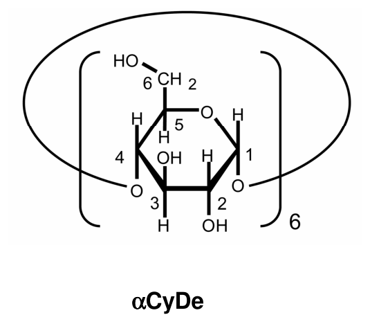
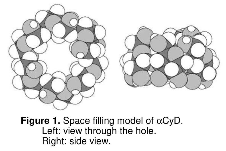
Figure 1. Space filling model of αCyD.
Left: view through the hole.
Right: side view.
9.1 Give the absolute configuration (\(R\) or \(S\)) at stereogenic carbons C-2 and C-5 of D-glucose. Also, draw a stereostructure of the open chain form of D-glucose.
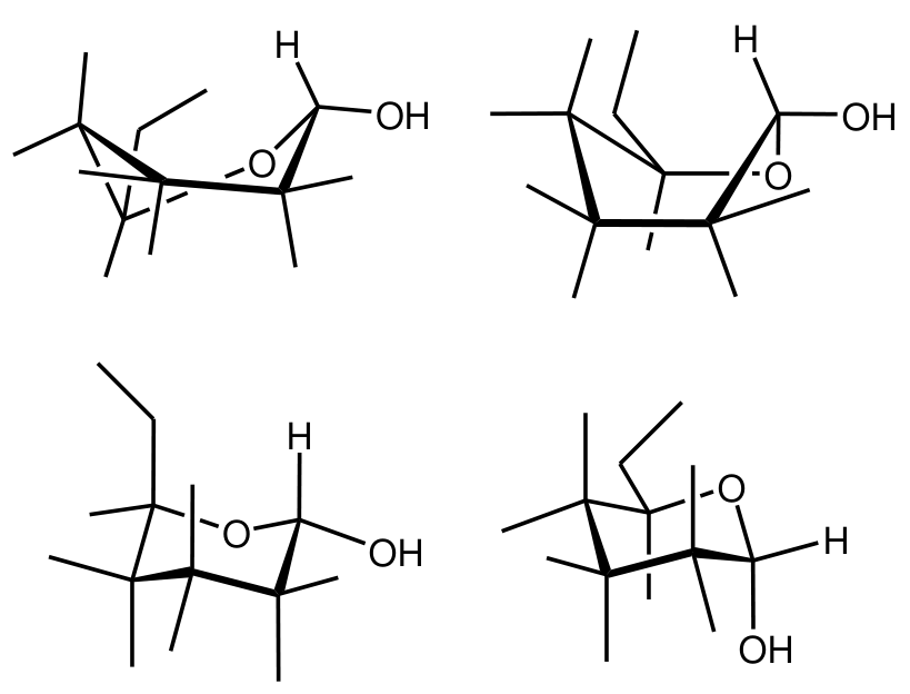
9.2 Choose the most stable conformation from the following four incomplete α-D-glucopyranose formulas. Also, add four \(\ce{OH}\) groups and four \(\ce{H}\) atoms to complete the α-D-glucopyranose formula.
αCyD in water is able to host hydrophobic molecules. When the host : guest (H : G) stoichiometry is 1 : 1, the inclusion complexation can be given by the following equilibrium.
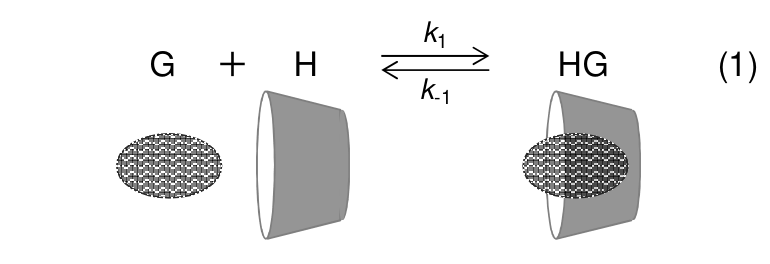
where \(k_1\) and \(k_{-1}\) are the rate constant for the forward and backward reaction, respectively. The complexation of a guest to αCyD causes a chemical shift change in \(\ce{^1H}\) NMR spectra.
Figure 2 shows a part of \(\ce{^1H}\) NMR spectra (signals from H–1 of αCyD) showing the chemical shift change in the presence of varying amounts of BTAD (1,10-bis(trimethylammonium)decane diiodide). The doublet peak at 5.06 ppm is from H–1 of free αCyD, while the doublet at 5.14 ppm is from H–1 of αCyD complexed with BTAD. (Note that the spectra given in Figure 2 were measured in the complexation equilibrium state.)
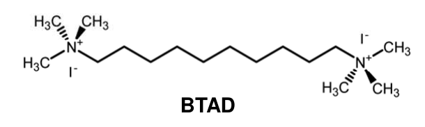
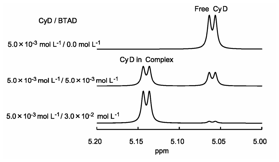
Figure 2.
Expanded \(\ce{^1H}\) NMR spectra (signals from H–1 of αCyD) of solutions with concentration of αCyD equal to \(5.0\cdot10^{-3}\ \mathrm{mol\,dm^{-3}}\) and that of BTAD equal from 0 to \(3.0\cdot10^{-2}\ \mathrm{mol\,dm^{-3}}\).
9.3 Consider a solution in which concentrations of αCyD as well as BTAD are equal to \(5.0\cdot10^{-3}\ \mathrm{mol\,dm^{-3}}\) and the relative peak areas of the doublets at 5.06 and 5.14 ppm are 0.41 and 0.59, respectively. Calculate (to 2 significant figures) the concentration equilibrium constant, \(K\), for the inclusion complexation of αCyD / BTAD.
Complexation of αCyD with hexyltrimethylammonium bromide (HTAB) appears in NMR spectra in a way different from the αCyD/BTAD complexation. Figure 3 shows a part of \(\ce{^1H}\) NMR spectra (H-6 signal of HTAB) in αCyD/HTAB solutions. The signal appears as one triplet (not two triplets), which shifts depending on the concentration of αCyD from the position of free HTAB to the position of αCyD/HTAB in proportion to the fraction of the complex in the solution. The H-6 signals from free HTAB and HTAB complexed with αCyD are triplets at 0.740 ppm and 0.860 ppm, respectively.
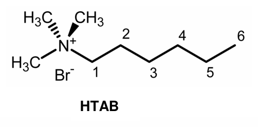
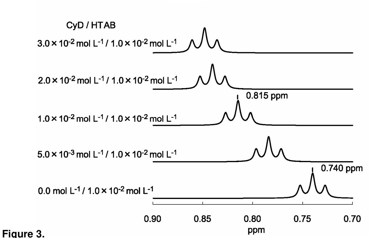
Figure 3.
Expanded \(\ce{^1H}\) NMR spectra (H-6 signal of HTAB) of solutions with concentration of HTAB equal to \(1.0\cdot10^{-2}\ \mathrm{mol\,dm^{-3}}\) and that of αCyD equal from 0 to \(3.0\cdot10^{-2}\ \mathrm{mol\,dm^{-3}}\).
9.4 The signal of HTAB in αCyD/HTAB solutions appears as one triplet that shifts depending on the concentration of αCyD. Choose the rational interpretation(s) just from these spectra.
Hint: When a guest molecule move in and out of αCyD rapidly and repeatedly, only one signal of the guest is observed at the weighted average of the chemical shifts of the free guest and the shift of the guest included in αCyD.
a) \(k_1\) of αCyD/HTAB \(>\) \(k_1\) of αCyD/BTAD
b) \(k_1\) of αCyD/HTAB \(<\) \(k_1\) of αCyD/BTAD
c) \(K\) of αCyD/HTAB \(>\) \(K\) of αCyD/BTAD
d) \(K\) of αCyD/HTAB \(<\) \(K\) of αCyD/BTAD
9.5 The signals of HTAB in the solution with concentrations of αCyD as well as HTAB equal to \(1.0\cdot10^{-2}\ \mathrm{mol\,dm^{-3}}\) are positioned at 0.815 ppm. Calculate (to 2 significant figures) the value of \(K\) for the complexation of αCyD/HTAB.
9.6 At 40.0 °C and 60.0 °C, \(K\) for the complexation of αCyD / HTAB are \(3.12\cdot10^2\) and \(2.09\cdot10^2\) respectively. Calculate (to 2 significant figures) the enthalpy change, \(\Delta H^\circ\) [\(\mathrm{kJ\,mol^{-1}}\)] and the entropy change, \(\Delta S^\circ\) [\(\mathrm{J\,K^{-1}\,mol^{-1}}\)]. (Ignore the temperature dependence of \(\Delta H^\circ\) and \(\Delta S^\circ\).)
Official English text of the problem.
Answers
- 9.1: C-2: \(R\); C-5: \(R\). Open-chain D-glucose:
O=C[C@H](O)[C@@H](O)[C@H](O)[C@H](O)CO. Its Fischer projection has \(\ce{CHO}\) at the top, \(\ce{CH2OH}\) at the bottom, and the \(\ce{OH}\) groups at C-2 through C-5 right, left, right, right. - 9.2: Choose the lower-right structure, the \(^{4}C_1\) chair of α-D-glucopyranose:
OC[C@H]1O[C@H](O)[C@H](O)[C@@H](O)[C@@H]1O. The C-1 \(\ce{OH}\) is axial down; the C-2, C-3 and C-4 \(\ce{OH}\) groups and C-5 \(\ce{CH2OH}\) group are equatorial. Complete the labels as specified below. - 9.3: \(\boxed{K_{\mathrm{BTAD}}=7.0\times10^2\ \mathrm{dm^3\,mol^{-1}}}\).
- 9.4: a) is the intended qualitative interpretation of the exchange pattern. The quantitative population data also establish d); see the qualification below.
- 9.5: \(\boxed{K_{\mathrm{HTAB}}=4.4\times10^2\ \mathrm{dm^3\,mol^{-1}}}\).
- 9.6: \(\boxed{\Delta H^\circ=-17\ \mathrm{kJ\,mol^{-1}}}\), \(\boxed{\Delta S^\circ=-7.7\ \mathrm{J\,K^{-1}\,mol^{-1}}}\).
Solution
9.1
The required Fischer projection of open-chain D-glucose has the carbon chain vertical, with the aldehyde group \(\ce{CHO}\) uppermost and \(\ce{CH2OH}\) at the bottom.
| Stereogenic carbon | Left-hand substituent | Right-hand substituent |
|---|---|---|
| C-2 | \(\ce{H}\) | \(\ce{OH}\) |
| C-3 | \(\ce{OH}\) | \(\ce{H}\) |
| C-4 | \(\ce{H}\) | \(\ce{OH}\) |
| C-5 | \(\ce{H}\) | \(\ce{OH}\) |
In a Fischer projection, horizontal bonds point towards the viewer and vertical bonds point away.
At C-2, the CIP priorities are
\[ \ce{OH} > \text{C-1 side} > \text{C-3 side} > \ce{H}. \]
The aldehyde carbon is compared as attached to \((\ce{O},\ce{O},\ce{H})\), whereas C-3 is attached to \((\ce{O},\ce{C},\ce{H})\). Therefore the aldehyde side has higher priority. Accounting for the horizontal hydrogen pointing towards the viewer gives \(R\).
At C-5, the priorities are
\[ \ce{OH} > \text{C-4 side} > \ce{CH2OH} > \ce{H}. \]
The C-4 side has attached atoms \((\ce{O},\ce{C},\ce{H})\), whereas C-6 has \((\ce{O},\ce{H},\ce{H})\). The same Fischer-projection analysis gives \(R\).
Thus
\[ \boxed{\text{C-2: }R,\qquad \text{C-5: }R}. \]
The complete open-chain configuration is \((2R,3S,4R,5R)\).
9.2
The lower-right drawing is the stable \(^{4}C_1\) chair. Complete it according to this table; “up” and “down” refer to the two faces of the ring.
| Carbon | Oxygen-containing substituent | Hydrogen |
|---|---|---|
| C-1 | \(\ce{OH}\): axial, down | Equatorial, up |
| C-2 | \(\ce{OH}\): equatorial, down | Axial, up |
| C-3 | \(\ce{OH}\): equatorial, up | Axial, down |
| C-4 | \(\ce{OH}\): equatorial, down | Axial, up |
| C-5 | \(\ce{CH2OH}\): equatorial, up | Axial, down |
Specifically, add the four missing \(\ce{OH}\) labels at C-2, C-3, C-4, and the end of the C-6 side chain. Add the four missing \(\ce{H}\) labels at C-2, C-3, C-4, and C-5.
This chair places the three non-anomeric ring hydroxyl groups and the hydroxymethyl group equatorial, minimizing unfavorable axial interactions. For the α anomer, the anomeric hydroxyl group is on the opposite face from the C-5 hydroxymethyl group, so it is axial down in this chair.
The SMILES given above specifies the stereoisomer; the chair conformation and axial/equatorial placements are specified by the table.
9.3
Let H denote the host, G the guest, and HG their 1:1 inclusion complex:
\[ \ce{H + G <=> HG}. \]
The concentration equilibrium constant is
\[ K=\frac{[\mathrm{HG}]}{[\mathrm H][\mathrm G]}. \]
Each free or complexed host contributes the same number of H–1 protons. Consequently, the integrated peak areas give the fractions of host in the two states:
\[ f_{\mathrm{free}}=0.41,\qquad f_{\mathrm{complexed}}=0.59. \]
With total host and guest concentrations both equal to \(5.0\times10^{-3}\ \mathrm{mol\,dm^{-3}}\),
\[ [\mathrm{HG}] =0.59(5.0\times10^{-3}) =2.95\times10^{-3}\ \mathrm{mol\,dm^{-3}}, \]
\[ [\mathrm H] =0.41(5.0\times10^{-3}) =2.05\times10^{-3}\ \mathrm{mol\,dm^{-3}}. \]
The 1:1 stoichiometry and equal total concentrations give
\[ [\mathrm G] =5.0\times10^{-3}-2.95\times10^{-3} =2.05\times10^{-3}\ \mathrm{mol\,dm^{-3}}. \]
Therefore,
\[ K_{\mathrm{BTAD}} =\frac{2.95\times10^{-3}} {(2.05\times10^{-3})^2} =701.96\ \mathrm{dm^3\,mol^{-1}}, \]
or, to two significant figures,
\[ \boxed{K_{\mathrm{BTAD}}=7.0\times10^2\ \mathrm{dm^3\,mol^{-1}}}. \]
9.4
For HTAB, the single triplet at an intermediate chemical shift indicates rapid exchange between free and bound states on the NMR timescale. Its observed shift is
\[ \delta_{\mathrm{obs}} =(1-f)\delta_{\mathrm{free}}+f\delta_{\mathrm{bound}}, \]
where \(f\) is the fraction of guest bound.
For BTAD, separate free-host and complexed-host doublets remain visible, indicating slow exchange on the NMR timescale.
The intended qualitative kinetic interpretation is therefore a): faster association/exchange for HTAB.
An averaged signal does not itself establish stronger or weaker equilibrium binding. At equilibrium,
\[ k_1[\mathrm H][\mathrm G]=k_{-1}[\mathrm{HG}], \qquad K=\frac{k_1}{k_{-1}}. \]
Both forward and reverse exchange can become faster without increasing their ratio. Thus neither c) nor d) follows merely from the distinction between averaged and separate signals.
Using the quantitative populations, however, parts 9.3 and 9.5 establish
\[ K_{\mathrm{HTAB}}<K_{\mathrm{BTAD}}, \]
so d) is also supported when the numerical information in the spectra is included.
9.5
Let \(f\) be the fraction of HTAB present in the complex. The weighted-average shift gives
\[ 0.815=(1-f)(0.740)+f(0.860). \]
Hence
\[ f=\frac{0.815-0.740}{0.860-0.740} =\frac{0.075}{0.120} =0.625. \]
The total guest concentration is \(1.0\times10^{-2}\ \mathrm{mol\,dm^{-3}}\), so
\[ [\mathrm{HG}] =0.625(1.0\times10^{-2}) =6.25\times10^{-3}\ \mathrm{mol\,dm^{-3}}. \]
Because the total host and guest concentrations are equal,
\[ [\mathrm H]=[\mathrm G] =1.0\times10^{-2}-6.25\times10^{-3} =3.75\times10^{-3}\ \mathrm{mol\,dm^{-3}}. \]
Therefore,
\[ K_{\mathrm{HTAB}} =\frac{6.25\times10^{-3}} {(3.75\times10^{-3})^2} =444.44\ \mathrm{dm^3\,mol^{-1}}, \]
giving
\[ \boxed{K_{\mathrm{HTAB}}=4.4\times10^2\ \mathrm{dm^3\,mol^{-1}}}. \]
9.6
Convert the temperatures to kelvin:
\[ T_1=313.15\ \mathrm K,\qquad T_2=333.15\ \mathrm K. \]
For thermodynamic logarithms, use the dimensionless constant \(K^\circ=Kc^\circ\), with \(c^\circ=1\ \mathrm{mol\,dm^{-3}}\). Its numerical values are therefore 312 and 209.
Assuming temperature-independent \(\Delta H^\circ\), the integrated van ’t Hoff equation is
\[ \ln\left(\frac{K_2^\circ}{K_1^\circ}\right) =-\frac{\Delta H^\circ}{R} \left(\frac1{T_2}-\frac1{T_1}\right). \]
Using \(R=8.31446\ \mathrm{J\,K^{-1}\,mol^{-1}}\),
\[ \Delta H^\circ = -\frac{R\ln(209/312)} {1/333.15-1/313.15} =-1.73773\times10^4\ \mathrm{J\,mol^{-1}}. \]
Thus
\[ \boxed{\Delta H^\circ=-17\ \mathrm{kJ\,mol^{-1}}}. \]
The negative sign agrees with the decrease of \(K\) as temperature increases.
Next,
\[ \Delta G^\circ=-RT\ln K^\circ =\Delta H^\circ-T\Delta S^\circ, \]
so
\[ \Delta S^\circ=R\ln K^\circ+\frac{\Delta H^\circ}{T}. \]
Using \(T_1\) and retaining the unrounded enthalpy,
\[ \Delta S^\circ =(8.31446)\ln312 +\frac{-17377.3}{313.15} =-7.7419\ \mathrm{J\,K^{-1}\,mol^{-1}}. \]
Therefore,
\[ \boxed{\Delta S^\circ=-7.7\ \mathrm{J\,K^{-1}\,mol^{-1}}}. \]
The solution was checked against the official solution.
IChO 2010 · Theorieaufgabe 9
α-Cyclodextrin
α-Cyclodextrin (αCyD), ein cyclisches Oligosaccharid aus sechs α(1→4)-verknüpften α-D-Glucopyranosid-Einheiten, lässt sich topologisch als Torus darstellen (Abbildung 1). Die α-D-Glucopyranosid-Einheiten in αCyD liegen gewöhnlich in der stabilsten Sesselkonformation vor.
Abbildung 1. Kalottenmodell von αCyD.
Links: Blick durch den Hohlraum.
Rechts: Seitenansicht.
9.1 Geben Sie die absolute Konfiguration (\(R\) oder \(S\)) an den stereogenen Kohlenstoffatomen C-2 und C-5 der D-Glucose an. Zeichnen Sie außerdem eine stereochemische Strukturformel der offenkettigen Form der D-Glucose.
9.2 Wählen Sie aus den folgenden vier unvollständigen Formeln der α-D-Glucopyranose die stabilste Konformation aus. Ergänzen Sie außerdem vier \(\ce{OH}\)-Gruppen und vier \(\ce{H}\)-Atome, um die Formel der α-D-Glucopyranose zu vervollständigen.
αCyD kann in Wasser hydrophobe Moleküle als Gäste aufnehmen. Bei einer Wirt : Gast (H : G)-Stöchiometrie von 1 : 1 lässt sich die Bildung des Einschlusskomplexes durch das folgende Gleichgewicht beschreiben.
Dabei sind \(k_1\) und \(k_{-1}\) die Geschwindigkeitskonstanten der Hin- bzw. Rückreaktion. Die Komplexierung eines Gastes durch αCyD bewirkt eine Änderung der chemischen Verschiebung in \(\ce{^1H}\)-NMR-Spektren.
Abbildung 2 zeigt einen Ausschnitt aus \(\ce{^1H}\)-NMR-Spektren (Signale von H–1 des αCyD), der die Änderung der chemischen Verschiebung in Gegenwart unterschiedlicher Mengen BTAD (1,10-Bis(trimethylammonium)decan-diiodid) zeigt. Das Dublett bei 5.06 ppm stammt von H–1 des freien αCyD, während das Dublett bei 5.14 ppm von H–1 des mit BTAD komplexierten αCyD stammt. (Beachten Sie, dass die in Abbildung 2 dargestellten Spektren im Komplexierungsgleichgewicht aufgenommen wurden.)
Abbildung 2.
Vergrößerte Ausschnitte aus \(\ce{^1H}\)-NMR-Spektren (Signale von H–1 des αCyD) von Lösungen mit einer αCyD-Konzentration von \(5.0\cdot10^{-3}\ \mathrm{mol\,dm^{-3}}\) und BTAD-Konzentrationen von 0 bis \(3.0\cdot10^{-2}\ \mathrm{mol\,dm^{-3}}\).
9.3 Betrachten Sie eine Lösung, in der die Konzentrationen sowohl von αCyD als auch von BTAD \(5.0\cdot10^{-3}\ \mathrm{mol\,dm^{-3}}\) betragen und die relativen Peakflächen der Dubletts bei 5.06 bzw. 5.14 ppm 0.41 bzw. 0.59 sind. Berechnen Sie (auf 2 signifikante Stellen) die Konzentrationsgleichgewichtskonstante \(K\) für die Bildung des Einschlusskomplexes αCyD / BTAD.
Die Komplexierung von αCyD mit Hexyltrimethylammoniumbromid (HTAB) zeigt sich in NMR-Spektren auf andere Weise als die αCyD/BTAD-Komplexierung. Abbildung 3 zeigt einen Ausschnitt aus \(\ce{^1H}\)-NMR-Spektren (H-6-Signal von HTAB) in αCyD/HTAB-Lösungen. Das Signal erscheint als ein Triplett (nicht als zwei Tripletts), das sich abhängig von der αCyD-Konzentration proportional zum Anteil des Komplexes in der Lösung von der Position des freien HTAB zur Position von αCyD/HTAB verschiebt. Die H-6-Signale des freien HTAB und des mit αCyD komplexierten HTAB sind Tripletts bei 0.740 bzw. 0.860 ppm.
Abbildung 3.
Vergrößerte Ausschnitte aus \(\ce{^1H}\)-NMR-Spektren (H-6-Signal von HTAB) von Lösungen mit einer HTAB-Konzentration von \(1.0\cdot10^{-2}\ \mathrm{mol\,dm^{-3}}\) und αCyD-Konzentrationen von 0 bis \(3.0\cdot10^{-2}\ \mathrm{mol\,dm^{-3}}\).
9.4 Das Signal von HTAB in αCyD/HTAB-Lösungen erscheint als ein Triplett, das sich abhängig von der αCyD-Konzentration verschiebt. Wählen Sie die allein anhand dieser Spektren begründbare(n) Interpretation(en) aus.
Hinweis: Wenn sich ein Gastmolekül schnell und wiederholt in αCyD hinein- und wieder herausbewegt, wird nur ein Signal des Gastes beim gewichteten Mittelwert der chemischen Verschiebungen des freien Gastes und des in αCyD eingeschlossenen Gastes beobachtet.
a) \(k_1\) von αCyD/HTAB \(>\) \(k_1\) von αCyD/BTAD
b) \(k_1\) von αCyD/HTAB \(<\) \(k_1\) von αCyD/BTAD
c) \(K\) von αCyD/HTAB \(>\) \(K\) von αCyD/BTAD
d) \(K\) von αCyD/HTAB \(<\) \(K\) von αCyD/BTAD
9.5 Die Signale von HTAB in der Lösung, in der die Konzentrationen sowohl von αCyD als auch von HTAB \(1.0\cdot10^{-2}\ \mathrm{mol\,dm^{-3}}\) betragen, liegen bei 0.815 ppm. Berechnen Sie (auf 2 signifikante Stellen) den Wert von \(K\) für die Komplexierung von αCyD/HTAB.
9.6 Bei 40.0 °C und 60.0 °C beträgt \(K\) für die Komplexierung von αCyD / HTAB \(3.12\cdot10^2\) bzw. \(2.09\cdot10^2\). Berechnen Sie (auf 2 signifikante Stellen) die Enthalpieänderung \(\Delta H^\circ\) [\(\mathrm{kJ\,mol^{-1}}\)] und die Entropieänderung \(\Delta S^\circ\) [\(\mathrm{J\,K^{-1}\,mol^{-1}}\)]. (Vernachlässigen Sie die Temperaturabhängigkeit von \(\Delta H^\circ\) und \(\Delta S^\circ\).)
Aufgabentext aus dem offiziellen englischen Text übersetzt.
Antworten
- 9.1: C-2: \(R\); C-5: \(R\). Offenkettige D-Glucose:
O=C[C@H](O)[C@@H](O)[C@H](O)[C@H](O)CO. In ihrer Fischer-Projektion steht \(\ce{CHO}\) oben und \(\ce{CH2OH}\) unten; die \(\ce{OH}\)-Gruppen an C-2 bis C-5 stehen rechts, links, rechts, rechts. - 9.2: Wählen Sie die Struktur unten rechts, den \(^{4}C_1\)-Sessel der α-D-Glucopyranose:
OC[C@H]1O[C@H](O)[C@H](O)[C@@H](O)[C@@H]1O. Die \(\ce{OH}\)-Gruppe an C-1 steht axial nach unten; die \(\ce{OH}\)-Gruppen an C-2, C-3 und C-4 sowie die \(\ce{CH2OH}\)-Gruppe an C-5 stehen äquatorial. Vervollständigen Sie die Beschriftung wie unten angegeben. - 9.3: \(\boxed{K_{\mathrm{BTAD}}=7.0\times10^2\ \mathrm{dm^3\,mol^{-1}}}\).
- 9.4: a) ist die beabsichtigte qualitative Interpretation des Austauschmusters. Die quantitativen Daten zu den Anteilen der Spezies belegen auch d); siehe die nachstehende Einschränkung.
- 9.5: \(\boxed{K_{\mathrm{HTAB}}=4.4\times10^2\ \mathrm{dm^3\,mol^{-1}}}\).
- 9.6: \(\boxed{\Delta H^\circ=-17\ \mathrm{kJ\,mol^{-1}}}\), \(\boxed{\Delta S^\circ=-7.7\ \mathrm{J\,K^{-1}\,mol^{-1}}}\).
Lösung
9.1
In der geforderten Fischer-Projektion der offenkettigen D-Glucose verläuft die Kohlenstoffkette senkrecht, mit der Aldehydgruppe \(\ce{CHO}\) ganz oben und \(\ce{CH2OH}\) unten.
| Stereogenes Kohlenstoffatom | Linker Substituent | Rechter Substituent |
|---|---|---|
| C-2 | \(\ce{H}\) | \(\ce{OH}\) |
| C-3 | \(\ce{OH}\) | \(\ce{H}\) |
| C-4 | \(\ce{H}\) | \(\ce{OH}\) |
| C-5 | \(\ce{H}\) | \(\ce{OH}\) |
In einer Fischer-Projektion zeigen waagerechte Bindungen zum Betrachter hin und senkrechte Bindungen vom Betrachter weg.
An C-2 lauten die CIP-Prioritäten
\[ \ce{OH} > \text{C-1-Seite} > \text{C-3-Seite} > \ce{H}. \]
Beim Vergleich wird das Aldehyd-Kohlenstoffatom so behandelt, als sei es an \((\ce{O},\ce{O},\ce{H})\) gebunden, während C-3 an \((\ce{O},\ce{C},\ce{H})\) gebunden ist. Daher hat die Aldehydseite die höhere Priorität. Unter Berücksichtigung des waagerecht angeordneten, zum Betrachter zeigenden Wasserstoffatoms ergibt sich \(R\).
An C-5 lauten die Prioritäten
\[ \ce{OH} > \text{C-4-Seite} > \ce{CH2OH} > \ce{H}. \]
Auf der C-4-Seite sind die Atome \((\ce{O},\ce{C},\ce{H})\) gebunden, an C-6 dagegen \((\ce{O},\ce{H},\ce{H})\). Die gleiche Auswertung der Fischer-Projektion ergibt \(R\).
Somit gilt
\[ \boxed{\text{C-2: }R,\qquad \text{C-5: }R}. \]
Die vollständige Konfiguration der offenkettigen Form ist \((2R,3S,4R,5R)\).
9.2
Die Zeichnung unten rechts zeigt den stabilen \(^{4}C_1\)-Sessel. Vervollständigen Sie sie gemäß dieser Tabelle; „oben“ und „unten“ beziehen sich auf die beiden Seiten des Rings.
| Kohlenstoffatom | Sauerstoffhaltiger Substituent | Wasserstoff |
|---|---|---|
| C-1 | \(\ce{OH}\): axial, nach unten | Äquatorial, nach oben |
| C-2 | \(\ce{OH}\): äquatorial, nach unten | Axial, nach oben |
| C-3 | \(\ce{OH}\): äquatorial, nach oben | Axial, nach unten |
| C-4 | \(\ce{OH}\): äquatorial, nach unten | Axial, nach oben |
| C-5 | \(\ce{CH2OH}\): äquatorial, nach oben | Axial, nach unten |
Ergänzen Sie konkret die vier fehlenden \(\ce{OH}\)-Beschriftungen an C-2, C-3, C-4 und am Ende der C-6-Seitenkette. Ergänzen Sie die vier fehlenden \(\ce{H}\)-Beschriftungen an C-2, C-3, C-4 und C-5.
In dieser Sesselkonformation stehen die drei nicht-anomeren Hydroxygruppen am Ring und die Hydroxymethylgruppe äquatorial, wodurch ungünstige axiale Wechselwirkungen minimiert werden. Beim α-Anomer liegt die anomere Hydroxygruppe auf der gegenüberliegenden Seite der Hydroxymethylgruppe an C-5 und steht daher in dieser Sesselkonformation axial nach unten.
Die oben angegebene SMILES-Zeichenfolge legt das Stereoisomer fest; die Sesselkonformation und die axialen bzw. äquatorialen Positionen werden durch die Tabelle angegeben.
9.3
H bezeichne den Wirt, G den Gast und HG ihren 1:1-Einschlusskomplex:
\[ \ce{H + G <=> HG}. \]
Die Konzentrationsgleichgewichtskonstante ist
\[ K=\frac{[\mathrm{HG}]}{[\mathrm H][\mathrm G]}. \]
Jeder freie oder komplexierte Wirt trägt dieselbe Anzahl an H–1-Protonen bei. Daher ergeben die integrierten Peakflächen die Anteile des Wirts in den beiden Zuständen:
\[ f_{\mathrm{free}}=0.41,\qquad f_{\mathrm{complexed}}=0.59. \]
Bei Gesamtkonzentrationen von Wirt und Gast von jeweils \(5.0\times10^{-3}\ \mathrm{mol\,dm^{-3}}\) gilt
\[ [\mathrm{HG}] =0.59(5.0\times10^{-3}) =2.95\times10^{-3}\ \mathrm{mol\,dm^{-3}}, \]
\[ [\mathrm H] =0.41(5.0\times10^{-3}) =2.05\times10^{-3}\ \mathrm{mol\,dm^{-3}}. \]
Aus der 1:1-Stöchiometrie und den gleichen Gesamtkonzentrationen ergibt sich
\[ [\mathrm G] =5.0\times10^{-3}-2.95\times10^{-3} =2.05\times10^{-3}\ \mathrm{mol\,dm^{-3}}. \]
Daher gilt
\[ K_{\mathrm{BTAD}} =\frac{2.95\times10^{-3}} {(2.05\times10^{-3})^2} =701.96\ \mathrm{dm^3\,mol^{-1}}, \]
oder, auf zwei signifikante Stellen gerundet,
\[ \boxed{K_{\mathrm{BTAD}}=7.0\times10^2\ \mathrm{dm^3\,mol^{-1}}}. \]
9.4
Bei HTAB weist das einzelne Triplett bei einer dazwischenliegenden chemischen Verschiebung auf einen schnellen Austausch zwischen freiem und gebundenem Zustand auf der NMR-Zeitskala hin. Seine beobachtete Verschiebung ist
\[ \delta_{\mathrm{obs}} =(1-f)\delta_{\mathrm{free}}+f\delta_{\mathrm{bound}}, \]
wobei \(f\) der Anteil des gebundenen Gastes ist.
Bei BTAD bleiben getrennte Dubletts des freien und des komplexierten Wirts sichtbar, was auf einen langsamen Austausch auf der NMR-Zeitskala hinweist.
Die beabsichtigte qualitative kinetische Interpretation ist daher a): schnellere Assoziation bzw. schnellerer Austausch bei HTAB.
Ein gemitteltes Signal allein belegt keine stärkere oder schwächere Bindung im Gleichgewicht. Im Gleichgewicht gilt
\[ k_1[\mathrm H][\mathrm G]=k_{-1}[\mathrm{HG}], \qquad K=\frac{k_1}{k_{-1}}. \]
Sowohl der Austausch in Hinrichtung als auch der in Rückrichtung kann schneller werden, ohne dass sich das Verhältnis der Geschwindigkeitskonstanten erhöht. Somit folgt weder c) noch d) allein aus dem Unterschied zwischen gemittelten und getrennten Signalen.
Unter Verwendung der quantitativen Anteile der Spezies belegen die Teilaufgaben 9.3 und 9.5 jedoch
\[ K_{\mathrm{HTAB}}<K_{\mathrm{BTAD}}, \]
sodass auch d) gestützt wird, wenn die numerischen Informationen aus den Spektren einbezogen werden.
9.5
Es sei \(f\) der Anteil des HTAB, der im Komplex vorliegt. Die als gewichteter Mittelwert erhaltene Verschiebung ergibt
\[ 0.815=(1-f)(0.740)+f(0.860). \]
Daraus folgt
\[ f=\frac{0.815-0.740}{0.860-0.740} =\frac{0.075}{0.120} =0.625. \]
Die Gesamtkonzentration des Gastes beträgt \(1.0\times10^{-2}\ \mathrm{mol\,dm^{-3}}\), somit gilt
\[ [\mathrm{HG}] =0.625(1.0\times10^{-2}) =6.25\times10^{-3}\ \mathrm{mol\,dm^{-3}}. \]
Da die Gesamtkonzentrationen von Wirt und Gast gleich sind, gilt
\[ [\mathrm H]=[\mathrm G] =1.0\times10^{-2}-6.25\times10^{-3} =3.75\times10^{-3}\ \mathrm{mol\,dm^{-3}}. \]
Daher gilt
\[ K_{\mathrm{HTAB}} =\frac{6.25\times10^{-3}} {(3.75\times10^{-3})^2} =444.44\ \mathrm{dm^3\,mol^{-1}}, \]
woraus sich ergibt
\[ \boxed{K_{\mathrm{HTAB}}=4.4\times10^2\ \mathrm{dm^3\,mol^{-1}}}. \]
9.6
Die Temperaturen werden in Kelvin umgerechnet:
\[ T_1=313.15\ \mathrm K,\qquad T_2=333.15\ \mathrm K. \]
Für die Logarithmen in den thermodynamischen Beziehungen wird die dimensionslose Konstante \(K^\circ=Kc^\circ\) mit \(c^\circ=1\ \mathrm{mol\,dm^{-3}}\) verwendet. Ihre Zahlenwerte sind daher 312 und 209.
Unter der Annahme eines temperaturunabhängigen \(\Delta H^\circ\) lautet die integrierte van-’t-Hoff-Gleichung
\[ \ln\left(\frac{K_2^\circ}{K_1^\circ}\right) =-\frac{\Delta H^\circ}{R} \left(\frac1{T_2}-\frac1{T_1}\right). \]
Mit \(R=8.31446\ \mathrm{J\,K^{-1}\,mol^{-1}}\) ergibt sich
\[ \Delta H^\circ = -\frac{R\ln(209/312)} {1/333.15-1/313.15} =-1.73773\times10^4\ \mathrm{J\,mol^{-1}}. \]
Somit gilt
\[ \boxed{\Delta H^\circ=-17\ \mathrm{kJ\,mol^{-1}}}. \]
Das negative Vorzeichen stimmt mit der Abnahme von \(K\) bei steigender Temperatur überein.
Weiter gilt
\[ \Delta G^\circ=-RT\ln K^\circ =\Delta H^\circ-T\Delta S^\circ, \]
also
\[ \Delta S^\circ=R\ln K^\circ+\frac{\Delta H^\circ}{T}. \]
Mit \(T_1\) und unter Beibehaltung des ungerundeten Enthalpiewerts ergibt sich
\[ \Delta S^\circ =(8.31446)\ln312 +\frac{-17377.3}{313.15} =-7.7419\ \mathrm{J\,K^{-1}\,mol^{-1}}. \]
Daher gilt
\[ \boxed{\Delta S^\circ=-7.7\ \mathrm{J\,K^{-1}\,mol^{-1}}}. \]
Die Lösung wurde mit der offiziellen Lösung abgeglichen.
IChO 2010 · Teori sorusu 9
α-Siklodekstrin
α(1→4) bağlarıyla bağlanmış altı α-D-glukopiranozit biriminden oluşan halkalı bir oligosakkarit olan α-siklodekstrin (αCyD), topolojik olarak toroit biçiminde gösterilebilir (Şekil 1). αCyD içindeki α-D-glukopiranozit birimleri genellikle en kararlı sandalye konformasyonundadır.
Şekil 1. αCyD'nin uzay dolduran modeli.
Sol: boşluk boyunca görünüm.
Sağ: yandan görünüm.
9.1 D-glukozun stereojenik C-2 ve C-5 karbonlarındaki mutlak konfigürasyonu (\(R\) veya \(S\)) belirtiniz. Ayrıca D-glukozun açık zincirli biçiminin stereoyapısını çiziniz.
9.2 Aşağıdaki tamamlanmamış dört α-D-glukopiranoz formülünden en kararlı konformasyonu seçiniz. Ayrıca α-D-glukopiranoz formülünü tamamlamak için dört \(\ce{OH}\) grubu ve dört \(\ce{H}\) atomu ekleyiniz.
αCyD, suda hidrofobik molekülleri konuk edebilir. Konak : konuk (H : G) stokiyometrisi 1 : 1 olduğunda, içerme kompleksi oluşumu aşağıdaki dengeyle gösterilebilir.
Burada \(k_1\) ve \(k_{-1}\), sırasıyla ileri ve geri tepkimelerin hız sabitleridir. Bir konuğun αCyD ile kompleks oluşturması, \(\ce{^1H}\) NMR spektrumlarında kimyasal kayma değişimine yol açar.
Şekil 2, değişen miktarlarda BTAD (1,10-bis(trimetilamonyum)dekan diiyodür) varlığındaki kimyasal kayma değişimini gösteren \(\ce{^1H}\) NMR spektrumlarının bir bölümünü (αCyD'nin H–1 sinyalleri) göstermektedir. 5.06 ppm'deki dublet pik serbest αCyD'nin H–1 protonundan, 5.14 ppm'deki dublet ise BTAD ile kompleks oluşturmuş αCyD'nin H–1 protonundan kaynaklanır. (Şekil 2'de verilen spektrumların kompleksleşme dengesi durumunda ölçüldüğüne dikkat ediniz.)
Şekil 2.
αCyD derişimi \(5.0\cdot10^{-3}\ \mathrm{mol\,dm^{-3}}\) olan ve BTAD derişimi 0 ile \(3.0\cdot10^{-2}\ \mathrm{mol\,dm^{-3}}\) arasında değişen çözeltilerin büyütülmüş \(\ce{^1H}\) NMR spektrumları (αCyD'nin H–1 sinyalleri).
9.3 Hem αCyD hem de BTAD derişiminin \(5.0\cdot10^{-3}\ \mathrm{mol\,dm^{-3}}\) olduğu ve 5.06 ile 5.14 ppm'deki dubletlerin bağıl pik alanlarının sırasıyla 0.41 ve 0.59 olduğu bir çözeltiyi ele alınız. αCyD / BTAD içerme kompleksi oluşumunun derişim cinsinden denge sabiti \(K\)'yi (2 anlamlı basamakla) hesaplayınız.
αCyD'nin heksiltrimetilamonyum bromür (HTAB) ile kompleksleşmesi, NMR spektrumlarında αCyD/BTAD kompleksleşmesinden farklı bir şekilde görünür. Şekil 3, αCyD/HTAB çözeltilerindeki \(\ce{^1H}\) NMR spektrumlarının bir bölümünü (HTAB'nin H-6 sinyali) göstermektedir. Sinyal, αCyD derişimine bağlı olarak serbest HTAB'nin konumundan αCyD/HTAB'nin konumuna, çözeltideki kompleksin kesriyle orantılı biçimde kayan tek bir triplet (iki triplet değil) olarak görünür. Serbest HTAB'nin ve αCyD ile kompleks oluşturmuş HTAB'nin H-6 sinyalleri, sırasıyla 0.740 ppm ve 0.860 ppm'de bulunan tripletlerdir.
Şekil 3.
HTAB derişimi \(1.0\cdot10^{-2}\ \mathrm{mol\,dm^{-3}}\) olan ve αCyD derişimi 0 ile \(3.0\cdot10^{-2}\ \mathrm{mol\,dm^{-3}}\) arasında değişen çözeltilerin büyütülmüş \(\ce{^1H}\) NMR spektrumları (HTAB'nin H-6 sinyali).
9.4 αCyD/HTAB çözeltilerindeki HTAB sinyali, αCyD derişimine bağlı olarak kayan tek bir triplet olarak görünür. Yalnızca bu spektrumlara dayanarak yapılabilecek mantıklı yorum(lar)ı seçiniz.
İpucu: Bir konuk molekül αCyD'nin içine hızla ve tekrar tekrar girip çıktığında, konuğun yalnızca tek bir sinyali gözlenir; bu sinyal, serbest konuğun kimyasal kayması ile αCyD içine alınmış konuğun kimyasal kaymasının ağırlıklı ortalamasında yer alır.
a) αCyD/HTAB'nin \(k_1\) değeri \(>\) αCyD/BTAD'nin \(k_1\) değeri
b) αCyD/HTAB'nin \(k_1\) değeri \(<\) αCyD/BTAD'nin \(k_1\) değeri
c) αCyD/HTAB'nin \(K\) değeri \(>\) αCyD/BTAD'nin \(K\) değeri
d) αCyD/HTAB'nin \(K\) değeri \(<\) αCyD/BTAD'nin \(K\) değeri
9.5 Hem αCyD hem de HTAB derişiminin \(1.0\cdot10^{-2}\ \mathrm{mol\,dm^{-3}}\) olduğu çözeltideki HTAB sinyalleri 0.815 ppm'de yer alır. αCyD/HTAB kompleksleşmesinin \(K\) değerini (2 anlamlı basamakla) hesaplayınız.
9.6 40.0 °C ve 60.0 °C'de αCyD / HTAB kompleksleşmesinin \(K\) değerleri sırasıyla \(3.12\cdot10^2\) ve \(2.09\cdot10^2\)'dir. Entalpi değişimini, \(\Delta H^\circ\) [\(\mathrm{kJ\,mol^{-1}}\)] ve entropi değişimini, \(\Delta S^\circ\) [\(\mathrm{J\,K^{-1}\,mol^{-1}}\)] (2 anlamlı basamakla) hesaplayınız. (\(\Delta H^\circ\) ve \(\Delta S^\circ\)'nin sıcaklığa bağımlılığını ihmal ediniz.)
Soru metni resmi İngilizce metinden çevrilmiştir.
Cevaplar
- 9.1: C-2: \(R\); C-5: \(R\). Açık zincirli D-glukoz:
O=C[C@H](O)[C@@H](O)[C@H](O)[C@H](O)CO. Fischer izdüşümünde üstte \(\ce{CHO}\), altta \(\ce{CH2OH}\) bulunur; C-2'den C-5'e kadar olan \(\ce{OH}\) grupları sırasıyla sağda, solda, sağda, sağdadır. - 9.2: Sağ alttaki yapıyı, α-D-glukopiranozun \(^{4}C_1\) sandalye konformasyonunu seçiniz:
OC[C@H]1O[C@H](O)[C@H](O)[C@@H](O)[C@@H]1O. C-1'deki \(\ce{OH}\) aksiyal ve aşağı yönlüdür; C-2, C-3 ve C-4'teki \(\ce{OH}\) grupları ile C-5'teki \(\ce{CH2OH}\) grubu ekvatoryaldir. Etiketleri aşağıda belirtildiği gibi tamamlayınız. - 9.3: \(\boxed{K_{\mathrm{BTAD}}=7.0\times10^2\ \mathrm{dm^3\,mol^{-1}}}\).
- 9.4: Değişim örüntüsünden çıkarılması amaçlanan nitel yorum a) seçeneğidir. Nicel popülasyon verileri d) seçeneğini de ortaya koyar; aşağıdaki açıklamaya bakınız.
- 9.5: \(\boxed{K_{\mathrm{HTAB}}=4.4\times10^2\ \mathrm{dm^3\,mol^{-1}}}\).
- 9.6: \(\boxed{\Delta H^\circ=-17\ \mathrm{kJ\,mol^{-1}}}\), \(\boxed{\Delta S^\circ=-7.7\ \mathrm{J\,K^{-1}\,mol^{-1}}}\).
Çözüm
9.1
Açık zincirli D-glukozun istenen Fischer izdüşümünde karbon zinciri düşeydir; aldehit grubu \(\ce{CHO}\) en üstte, \(\ce{CH2OH}\) ise en altta yer alır.
| Stereojenik karbon | Soldaki sübstitüent | Sağdaki sübstitüent |
|---|---|---|
| C-2 | \(\ce{H}\) | \(\ce{OH}\) |
| C-3 | \(\ce{OH}\) | \(\ce{H}\) |
| C-4 | \(\ce{H}\) | \(\ce{OH}\) |
| C-5 | \(\ce{H}\) | \(\ce{OH}\) |
Fischer izdüşümünde yatay bağlar gözlemciye doğru, düşey bağlar ise gözlemciden uzağa yönelir.
C-2'de CIP öncelikleri şöyledir:
\[ \ce{OH} > \text{C-1 tarafı} > \text{C-3 tarafı} > \ce{H}. \]
Karşılaştırmada aldehit karbonu \((\ce{O},\ce{O},\ce{H})\) atomlarına bağlı kabul edilirken C-3, \((\ce{O},\ce{C},\ce{H})\) atomlarına bağlıdır. Dolayısıyla aldehit tarafı daha yüksek önceliğe sahiptir. Yatay konumdaki hidrojenin gözlemciye doğru yöneldiği dikkate alındığında \(R\) elde edilir.
C-5'te öncelikler şöyledir:
\[ \ce{OH} > \text{C-4 tarafı} > \ce{CH2OH} > \ce{H}. \]
C-4 tarafında bağlı atomlar \((\ce{O},\ce{C},\ce{H})\) iken C-6'da \((\ce{O},\ce{H},\ce{H})\)'dir. Aynı Fischer izdüşümü analizi \(R\) sonucunu verir.
Böylece
\[ \boxed{\text{C-2: }R,\qquad \text{C-5: }R}. \]
Açık zincirli biçimin tam konfigürasyonu \((2R,3S,4R,5R)\)'dir.
9.2
Sağ alttaki çizim, kararlı \(^{4}C_1\) sandalye konformasyonudur. Çizimi aşağıdaki tabloya göre tamamlayınız; “yukarı” ve “aşağı” halkanın iki yüzünü ifade eder.
| Karbon | Oksijen içeren sübstitüent | Hidrojen |
|---|---|---|
| C-1 | \(\ce{OH}\): aksiyal, aşağı | Ekvatoryal, yukarı |
| C-2 | \(\ce{OH}\): ekvatoryal, aşağı | Aksiyal, yukarı |
| C-3 | \(\ce{OH}\): ekvatoryal, yukarı | Aksiyal, aşağı |
| C-4 | \(\ce{OH}\): ekvatoryal, aşağı | Aksiyal, yukarı |
| C-5 | \(\ce{CH2OH}\): ekvatoryal, yukarı | Aksiyal, aşağı |
Özellikle, eksik dört \(\ce{OH}\) etiketini C-2, C-3, C-4 ve C-6 yan zincirinin ucuna ekleyiniz. Eksik dört \(\ce{H}\) etiketini C-2, C-3, C-4 ve C-5'e ekleyiniz.
Bu sandalye konformasyonunda, halkadaki anomerik olmayan üç hidroksil grubu ve hidroksimetil grubu ekvatoryal konumda bulunur; böylece elverişsiz aksiyal etkileşimler en aza iner. α anomerinde anomerik hidroksil grubu, C-5'teki hidroksimetil grubuna göre halkanın karşı yüzündedir; bu nedenle bu sandalye konformasyonunda aksiyal ve aşağı yönlüdür.
Yukarıda verilen SMILES, stereoizomeri belirtir; sandalye konformasyonu ve aksiyal/ekvatoryal yerleşimler tabloda belirtilmiştir.
9.3
H konağı, G konuğu ve HG bunların 1:1 içerme kompleksini göstersin:
\[ \ce{H + G <=> HG}. \]
Derişim cinsinden denge sabiti şöyledir:
\[ K=\frac{[\mathrm{HG}]}{[\mathrm H][\mathrm G]}. \]
Serbest veya kompleksleşmiş her konak, aynı sayıda H–1 protonu katkısı yapar. Dolayısıyla piklerin integral alanları, konağın bu iki durumdaki kesirlerini verir:
\[ f_{\mathrm{free}}=0.41,\qquad f_{\mathrm{complexed}}=0.59. \]
Toplam konak ve konuk derişimlerinin her ikisi de \(5.0\times10^{-3}\ \mathrm{mol\,dm^{-3}}\) olduğundan,
\[ [\mathrm{HG}] =0.59(5.0\times10^{-3}) =2.95\times10^{-3}\ \mathrm{mol\,dm^{-3}}, \]
\[ [\mathrm H] =0.41(5.0\times10^{-3}) =2.05\times10^{-3}\ \mathrm{mol\,dm^{-3}}. \]
1:1 stokiyometrisi ve toplam derişimlerin eşit olması şu sonucu verir:
\[ [\mathrm G] =5.0\times10^{-3}-2.95\times10^{-3} =2.05\times10^{-3}\ \mathrm{mol\,dm^{-3}}. \]
Dolayısıyla,
\[ K_{\mathrm{BTAD}} =\frac{2.95\times10^{-3}} {(2.05\times10^{-3})^2} =701.96\ \mathrm{dm^3\,mol^{-1}}, \]
ya da iki anlamlı basamakla,
\[ \boxed{K_{\mathrm{BTAD}}=7.0\times10^2\ \mathrm{dm^3\,mol^{-1}}}. \]
9.4
HTAB için ara bir kimyasal kaymada gözlenen tek triplet, NMR zaman ölçeğinde serbest ve bağlı durumlar arasında hızlı değişim olduğunu gösterir. Gözlenen kimyasal kayma şöyledir:
\[ \delta_{\mathrm{obs}} =(1-f)\delta_{\mathrm{free}}+f\delta_{\mathrm{bound}}, \]
burada \(f\), konuğun bağlı olan kesridir.
BTAD için serbest konağa ve kompleksleşmiş konağa ait ayrı dubletler görünür olmaya devam eder; bu, NMR zaman ölçeğinde yavaş değişim olduğunu gösterir.
Dolayısıyla amaçlanan nitel kinetik yorum a) seçeneğidir: HTAB için daha hızlı birleşme/değişim.
Ortalamayı yansıtan bir sinyal, tek başına dengedeki bağlanmanın daha güçlü veya daha zayıf olduğunu ortaya koymaz. Dengede,
\[ k_1[\mathrm H][\mathrm G]=k_{-1}[\mathrm{HG}], \qquad K=\frac{k_1}{k_{-1}}. \]
İleri ve geri yöndeki değişimlerin her ikisi de, hız sabitlerinin oranı artmadan hızlanabilir. Bu nedenle yalnızca ortalamayı yansıtan sinyaller ile ayrı sinyaller arasındaki ayrımdan ne c) ne de d) sonucu çıkar.
Ancak nicel popülasyonlar kullanıldığında, 9.3 ve 9.5 kısımları
\[ K_{\mathrm{HTAB}}<K_{\mathrm{BTAD}}, \]
olduğunu ortaya koyar; dolayısıyla spektrumlardaki sayısal bilgiler hesaba katıldığında d) seçeneği de desteklenir.
9.5
\(f\), HTAB'nin kompleks içinde bulunan kesri olsun. Ağırlıklı ortalama kimyasal kayma şu bağıntıyı verir:
\[ 0.815=(1-f)(0.740)+f(0.860). \]
Buradan
\[ f=\frac{0.815-0.740}{0.860-0.740} =\frac{0.075}{0.120} =0.625. \]
Toplam konuk derişimi \(1.0\times10^{-2}\ \mathrm{mol\,dm^{-3}}\) olduğundan,
\[ [\mathrm{HG}] =0.625(1.0\times10^{-2}) =6.25\times10^{-3}\ \mathrm{mol\,dm^{-3}}. \]
Toplam konak ve konuk derişimleri eşit olduğu için,
\[ [\mathrm H]=[\mathrm G] =1.0\times10^{-2}-6.25\times10^{-3} =3.75\times10^{-3}\ \mathrm{mol\,dm^{-3}}. \]
Dolayısıyla,
\[ K_{\mathrm{HTAB}} =\frac{6.25\times10^{-3}} {(3.75\times10^{-3})^2} =444.44\ \mathrm{dm^3\,mol^{-1}}, \]
ve sonuç olarak
\[ \boxed{K_{\mathrm{HTAB}}=4.4\times10^2\ \mathrm{dm^3\,mol^{-1}}}. \]
9.6
Sıcaklıkları kelvine dönüştürelim:
\[ T_1=313.15\ \mathrm K,\qquad T_2=333.15\ \mathrm K. \]
Termodinamik logaritmalar için boyutsuz \(K^\circ=Kc^\circ\) sabitini kullanalım; burada \(c^\circ=1\ \mathrm{mol\,dm^{-3}}\)'tür. Dolayısıyla bu sabitin sayısal değerleri 312 ve 209'dur.
\(\Delta H^\circ\)'nin sıcaklıktan bağımsız olduğu varsayılırsa, integrali alınmış van ’t Hoff denklemi şöyledir:
\[ \ln\left(\frac{K_2^\circ}{K_1^\circ}\right) =-\frac{\Delta H^\circ}{R} \left(\frac1{T_2}-\frac1{T_1}\right). \]
\(R=8.31446\ \mathrm{J\,K^{-1}\,mol^{-1}}\) kullanılarak,
\[ \Delta H^\circ = -\frac{R\ln(209/312)} {1/333.15-1/313.15} =-1.73773\times10^4\ \mathrm{J\,mol^{-1}}. \]
Böylece
\[ \boxed{\Delta H^\circ=-17\ \mathrm{kJ\,mol^{-1}}}. \]
Negatif işaret, sıcaklık arttıkça \(K\)'nin azalmasıyla uyumludur.
Ardından,
\[ \Delta G^\circ=-RT\ln K^\circ =\Delta H^\circ-T\Delta S^\circ, \]
dolayısıyla
\[ \Delta S^\circ=R\ln K^\circ+\frac{\Delta H^\circ}{T}. \]
\(T_1\) kullanılıp entalpinin yuvarlanmamış değeri korunarak,
\[ \Delta S^\circ =(8.31446)\ln312 +\frac{-17377.3}{313.15} =-7.7419\ \mathrm{J\,K^{-1}\,mol^{-1}}. \]
Dolayısıyla,
\[ \boxed{\Delta S^\circ=-7.7\ \mathrm{J\,K^{-1}\,mol^{-1}}}. \]
Çözüm, resmi çözümle karşılaştırılarak kontrol edildi.
IChO 2010 · Problema teórico 9
α-Ciclodextrina
La α-ciclodextrina (αCyD), un oligosacárido cíclico formado por seis unidades de α-D-glucopiranósido unidas mediante enlaces α(1→4), puede representarse topológicamente como un toroide (Figura 1). Las unidades de α-D-glucopiranósido de la αCyD suelen adoptar la conformación de silla más estable.
Figura 1. Modelo de esferas de van der Waals de la αCyD.
Izquierda: vista a través del orificio.
Derecha: vista lateral.
9.1 Indique la configuración absoluta (\(R\) o \(S\)) de los carbonos estereogénicos C-2 y C-5 de la D-glucosa. Dibuje también una estructura que muestre la estereoquímica de la forma de cadena abierta de la D-glucosa.
9.2 Elija la conformación más estable entre las siguientes cuatro fórmulas incompletas de la α-D-glucopiranosa. Añada también cuatro grupos \(\ce{OH}\) y cuatro átomos de \(\ce{H}\) para completar la fórmula de la α-D-glucopiranosa.
La αCyD en agua puede alojar moléculas hidrófobas. Cuando la estequiometría anfitrión : huésped (H : G) es 1 : 1, la formación del complejo de inclusión puede expresarse mediante el siguiente equilibrio.
donde \(k_1\) y \(k_{-1}\) son las constantes de velocidad de las reacciones directa e inversa, respectivamente. La formación de un complejo entre un huésped y la αCyD provoca una variación del desplazamiento químico en los espectros de RMN de \(\ce{^1H}\).
La Figura 2 muestra una parte de los espectros de RMN de \(\ce{^1H}\) (señales de H–1 de la αCyD) que ilustra la variación del desplazamiento químico en presencia de distintas cantidades de BTAD (diyoduro de 1,10-bis(trimetilamonio)decano). El doblete a 5.06 ppm corresponde a H–1 de la αCyD libre, mientras que el doblete a 5.14 ppm corresponde a H–1 de la αCyD complejada con BTAD. (Tenga en cuenta que los espectros de la Figura 2 se midieron en el estado de equilibrio de formación del complejo.)
Figura 2.
Ampliación de los espectros de RMN de \(\ce{^1H}\) (señales de H–1 de la αCyD) de disoluciones con una concentración de αCyD igual a \(5.0\cdot10^{-3}\ \mathrm{mol\,dm^{-3}}\) y una concentración de BTAD comprendida entre 0 y \(3.0\cdot10^{-2}\ \mathrm{mol\,dm^{-3}}\).
9.3 Considere una disolución en la que las concentraciones tanto de αCyD como de BTAD son iguales a \(5.0\cdot10^{-3}\ \mathrm{mol\,dm^{-3}}\) y las áreas relativas de los dobletes a 5.06 y 5.14 ppm son 0.41 y 0.59, respectivamente. Calcule (con 2 cifras significativas) la constante de equilibrio en concentraciones, \(K\), para la formación del complejo de inclusión αCyD / BTAD.
La formación del complejo de αCyD con bromuro de hexiltrimetilamonio (HTAB) se manifiesta en los espectros de RMN de una manera distinta a la formación del complejo αCyD/BTAD. La Figura 3 muestra una parte de los espectros de RMN de \(\ce{^1H}\) (señal de H-6 del HTAB) en disoluciones de αCyD/HTAB. La señal aparece como un único triplete (no como dos tripletes), que se desplaza, en función de la concentración de αCyD, desde la posición del HTAB libre hasta la posición del αCyD/HTAB en proporción a la fracción de complejo en la disolución. Las señales de H-6 del HTAB libre y del HTAB complejado con αCyD son tripletes a 0.740 ppm y 0.860 ppm, respectivamente.
Figura 3.
Ampliación de los espectros de RMN de \(\ce{^1H}\) (señal de H-6 del HTAB) de disoluciones con una concentración de HTAB igual a \(1.0\cdot10^{-2}\ \mathrm{mol\,dm^{-3}}\) y una concentración de αCyD comprendida entre 0 y \(3.0\cdot10^{-2}\ \mathrm{mol\,dm^{-3}}\).
9.4 La señal del HTAB en las disoluciones de αCyD/HTAB aparece como un único triplete que se desplaza en función de la concentración de αCyD. Elija la interpretación o las interpretaciones razonables basándose únicamente en estos espectros.
Pista: Cuando una molécula huésped entra y sale de la αCyD de forma rápida y repetida, solo se observa una señal del huésped en el promedio ponderado de los desplazamientos químicos del huésped libre y del huésped incluido en la αCyD.
a) \(k_1\) de αCyD/HTAB \(>\) \(k_1\) de αCyD/BTAD
b) \(k_1\) de αCyD/HTAB \(<\) \(k_1\) de αCyD/BTAD
c) \(K\) de αCyD/HTAB \(>\) \(K\) de αCyD/BTAD
d) \(K\) de αCyD/HTAB \(<\) \(K\) de αCyD/BTAD
9.5 Las señales del HTAB en la disolución con concentraciones tanto de αCyD como de HTAB iguales a \(1.0\cdot10^{-2}\ \mathrm{mol\,dm^{-3}}\) se encuentran a 0.815 ppm. Calcule (con 2 cifras significativas) el valor de \(K\) para la formación del complejo αCyD/HTAB.
9.6 A 40.0 °C y 60.0 °C, los valores de \(K\) para la formación del complejo αCyD / HTAB son \(3.12\cdot10^2\) y \(2.09\cdot10^2\), respectivamente. Calcule (con 2 cifras significativas) la variación de entalpía, \(\Delta H^\circ\) [\(\mathrm{kJ\,mol^{-1}}\)], y la variación de entropía, \(\Delta S^\circ\) [\(\mathrm{J\,K^{-1}\,mol^{-1}}\)]. (Ignore la dependencia de \(\Delta H^\circ\) y \(\Delta S^\circ\) con la temperatura.)
Enunciado traducido del texto oficial en inglés.
Respuestas
- 9.1: C-2: \(R\); C-5: \(R\). D-glucosa de cadena abierta:
O=C[C@H](O)[C@@H](O)[C@H](O)[C@H](O)CO. Su proyección de Fischer tiene \(\ce{CHO}\) en la parte superior, \(\ce{CH2OH}\) en la parte inferior y los grupos \(\ce{OH}\) de C-2 a C-5 a la derecha, izquierda, derecha, derecha. - 9.2: Elija la estructura inferior derecha, la silla \(^{4}C_1\) de la α-D-glucopiranosa:
OC[C@H]1O[C@H](O)[C@H](O)[C@@H](O)[C@@H]1O. El \(\ce{OH}\) de C-1 es axial y apunta hacia abajo; los grupos \(\ce{OH}\) de C-2, C-3 y C-4 y el grupo \(\ce{CH2OH}\) de C-5 son ecuatoriales. Complete las etiquetas como se indica más adelante. - 9.3: \(\boxed{K_{\mathrm{BTAD}}=7.0\times10^2\ \mathrm{dm^3\,mol^{-1}}}\).
- 9.4: a) es la interpretación cualitativa que se pretende obtener del patrón de intercambio. Los datos cuantitativos de las poblaciones también permiten establecer d); véase la matización más adelante.
- 9.5: \(\boxed{K_{\mathrm{HTAB}}=4.4\times10^2\ \mathrm{dm^3\,mol^{-1}}}\).
- 9.6: \(\boxed{\Delta H^\circ=-17\ \mathrm{kJ\,mol^{-1}}}\), \(\boxed{\Delta S^\circ=-7.7\ \mathrm{J\,K^{-1}\,mol^{-1}}}\).
Solución
9.1
La proyección de Fischer solicitada para la D-glucosa de cadena abierta tiene la cadena carbonada en posición vertical, con el grupo aldehído \(\ce{CHO}\) en el extremo superior y \(\ce{CH2OH}\) en el inferior.
| Carbono estereogénico | Sustituyente a la izquierda | Sustituyente a la derecha |
|---|---|---|
| C-2 | \(\ce{H}\) | \(\ce{OH}\) |
| C-3 | \(\ce{OH}\) | \(\ce{H}\) |
| C-4 | \(\ce{H}\) | \(\ce{OH}\) |
| C-5 | \(\ce{H}\) | \(\ce{OH}\) |
En una proyección de Fischer, los enlaces horizontales apuntan hacia el observador y los verticales se alejan de él.
En C-2, las prioridades CIP son
\[ \ce{OH} > \text{lado de C-1} > \text{lado de C-3} > \ce{H}. \]
Al comparar prioridades, el carbono del aldehído se considera unido a \((\ce{O},\ce{O},\ce{H})\), mientras que C-3 está unido a \((\ce{O},\ce{C},\ce{H})\). Por tanto, el lado del aldehído tiene mayor prioridad. Al tener en cuenta que el hidrógeno horizontal apunta hacia el observador, se obtiene \(R\).
En C-5, las prioridades son
\[ \ce{OH} > \text{lado de C-4} > \ce{CH2OH} > \ce{H}. \]
El lado de C-4 tiene unidos los átomos \((\ce{O},\ce{C},\ce{H})\), mientras que C-6 tiene \((\ce{O},\ce{H},\ce{H})\). El mismo análisis de la proyección de Fischer da \(R\).
Así,
\[ \boxed{\text{C-2: }R,\qquad \text{C-5: }R}. \]
La configuración completa de la cadena abierta es \((2R,3S,4R,5R)\).
9.2
El dibujo inferior derecho corresponde a la silla estable \(^{4}C_1\). Complételo según esta tabla; «arriba» y «abajo» se refieren a las dos caras del anillo.
| Carbono | Sustituyente que contiene oxígeno | Hidrógeno |
|---|---|---|
| C-1 | \(\ce{OH}\): axial, abajo | Ecuatorial, arriba |
| C-2 | \(\ce{OH}\): ecuatorial, abajo | Axial, arriba |
| C-3 | \(\ce{OH}\): ecuatorial, arriba | Axial, abajo |
| C-4 | \(\ce{OH}\): ecuatorial, abajo | Axial, arriba |
| C-5 | \(\ce{CH2OH}\): ecuatorial, arriba | Axial, abajo |
En concreto, añada las cuatro etiquetas \(\ce{OH}\) que faltan en C-2, C-3, C-4 y el extremo de la cadena lateral de C-6. Añada las cuatro etiquetas \(\ce{H}\) que faltan en C-2, C-3, C-4 y C-5.
Esta silla sitúa los tres grupos hidroxilo no anoméricos del anillo y el grupo hidroximetilo en posiciones ecuatoriales, lo que minimiza las interacciones axiales desfavorables. En el anómero α, el grupo hidroxilo anomérico está en la cara opuesta a la del grupo hidroximetilo de C-5, por lo que es axial y apunta hacia abajo en esta silla.
La cadena SMILES indicada anteriormente especifica el estereoisómero; la conformación de silla y las posiciones axiales y ecuatoriales se especifican en la tabla.
9.3
Sean H el anfitrión, G el huésped y HG su complejo de inclusión 1:1:
\[ \ce{H + G <=> HG}. \]
La constante de equilibrio en concentraciones es
\[ K=\frac{[\mathrm{HG}]}{[\mathrm H][\mathrm G]}. \]
Cada anfitrión, libre o complejado, contribuye con el mismo número de protones H–1. Por consiguiente, las áreas integradas de los picos proporcionan las fracciones de anfitrión en los dos estados:
\[ f_{\mathrm{free}}=0.41,\qquad f_{\mathrm{complexed}}=0.59. \]
Con concentraciones totales de anfitrión y huésped ambas iguales a \(5.0\times10^{-3}\ \mathrm{mol\,dm^{-3}}\),
\[ [\mathrm{HG}] =0.59(5.0\times10^{-3}) =2.95\times10^{-3}\ \mathrm{mol\,dm^{-3}}, \]
\[ [\mathrm H] =0.41(5.0\times10^{-3}) =2.05\times10^{-3}\ \mathrm{mol\,dm^{-3}}. \]
La estequiometría 1:1 y la igualdad de las concentraciones totales dan
\[ [\mathrm G] =5.0\times10^{-3}-2.95\times10^{-3} =2.05\times10^{-3}\ \mathrm{mol\,dm^{-3}}. \]
Por tanto,
\[ K_{\mathrm{BTAD}} =\frac{2.95\times10^{-3}} {(2.05\times10^{-3})^2} =701.96\ \mathrm{dm^3\,mol^{-1}}, \]
o, con dos cifras significativas,
\[ \boxed{K_{\mathrm{BTAD}}=7.0\times10^2\ \mathrm{dm^3\,mol^{-1}}}. \]
9.4
Para el HTAB, el único triplete a un desplazamiento químico intermedio indica un intercambio rápido entre los estados libre y unido en la escala temporal de la RMN. Su desplazamiento observado es
\[ \delta_{\mathrm{obs}} =(1-f)\delta_{\mathrm{free}}+f\delta_{\mathrm{bound}}, \]
donde \(f\) es la fracción de huésped unido.
Para el BTAD, los dobletes del anfitrión libre y del anfitrión complejado siguen siendo visibles por separado, lo que indica un intercambio lento en la escala temporal de la RMN.
La interpretación cinética cualitativa que se pretende obtener es, por tanto, a): una asociación/un intercambio más rápidos para el HTAB.
Una señal promediada no permite establecer por sí sola si la unión en el equilibrio es más fuerte o más débil. En el equilibrio,
\[ k_1[\mathrm H][\mathrm G]=k_{-1}[\mathrm{HG}], \qquad K=\frac{k_1}{k_{-1}}. \]
Tanto el intercambio directo como el inverso pueden hacerse más rápidos sin que aumente el cociente entre sus constantes. Por ello, ni c) ni d) se deducen únicamente de la distinción entre señales promediadas y separadas.
Sin embargo, utilizando las poblaciones cuantitativas, los apartados 9.3 y 9.5 permiten establecer
\[ K_{\mathrm{HTAB}}<K_{\mathrm{BTAD}}, \]
por lo que d) también queda respaldada cuando se incluye la información numérica de los espectros.
9.5
Sea \(f\) la fracción de HTAB presente en el complejo. El desplazamiento promedio ponderado da
\[ 0.815=(1-f)(0.740)+f(0.860). \]
Por consiguiente,
\[ f=\frac{0.815-0.740}{0.860-0.740} =\frac{0.075}{0.120} =0.625. \]
La concentración total de huésped es \(1.0\times10^{-2}\ \mathrm{mol\,dm^{-3}}\), por lo que
\[ [\mathrm{HG}] =0.625(1.0\times10^{-2}) =6.25\times10^{-3}\ \mathrm{mol\,dm^{-3}}. \]
Como las concentraciones totales de anfitrión y huésped son iguales,
\[ [\mathrm H]=[\mathrm G] =1.0\times10^{-2}-6.25\times10^{-3} =3.75\times10^{-3}\ \mathrm{mol\,dm^{-3}}. \]
Por tanto,
\[ K_{\mathrm{HTAB}} =\frac{6.25\times10^{-3}} {(3.75\times10^{-3})^2} =444.44\ \mathrm{dm^3\,mol^{-1}}, \]
lo que da
\[ \boxed{K_{\mathrm{HTAB}}=4.4\times10^2\ \mathrm{dm^3\,mol^{-1}}}. \]
9.6
Convierta las temperaturas a kelvin:
\[ T_1=313.15\ \mathrm K,\qquad T_2=333.15\ \mathrm K. \]
Para los logaritmos termodinámicos, utilice la constante adimensional \(K^\circ=Kc^\circ\), con \(c^\circ=1\ \mathrm{mol\,dm^{-3}}\). Sus valores numéricos son, por tanto, 312 y 209.
Suponiendo que \(\Delta H^\circ\) no depende de la temperatura, la ecuación integrada de van ’t Hoff es
\[ \ln\left(\frac{K_2^\circ}{K_1^\circ}\right) =-\frac{\Delta H^\circ}{R} \left(\frac1{T_2}-\frac1{T_1}\right). \]
Utilizando \(R=8.31446\ \mathrm{J\,K^{-1}\,mol^{-1}}\),
\[ \Delta H^\circ = -\frac{R\ln(209/312)} {1/333.15-1/313.15} =-1.73773\times10^4\ \mathrm{J\,mol^{-1}}. \]
Así,
\[ \boxed{\Delta H^\circ=-17\ \mathrm{kJ\,mol^{-1}}}. \]
El signo negativo concuerda con la disminución de \(K\) al aumentar la temperatura.
A continuación,
\[ \Delta G^\circ=-RT\ln K^\circ =\Delta H^\circ-T\Delta S^\circ, \]
por lo que
\[ \Delta S^\circ=R\ln K^\circ+\frac{\Delta H^\circ}{T}. \]
Utilizando \(T_1\) y conservando el valor de la entalpía sin redondear,
\[ \Delta S^\circ =(8.31446)\ln312 +\frac{-17377.3}{313.15} =-7.7419\ \mathrm{J\,K^{-1}\,mol^{-1}}. \]
Por tanto,
\[ \boxed{\Delta S^\circ=-7.7\ \mathrm{J\,K^{-1}\,mol^{-1}}}. \]
La solución se comprobó con la solución oficial.
IChO 2010 · 理论题 9
α-环糊精
α-环糊精(αCyD)是由六个 α-D-吡喃葡萄糖苷单元通过 α(1→4) 键连接而成的环状低聚糖,其拓扑结构可表示为环面体(图 1)。αCyD 中的 α-D-吡喃葡萄糖苷单元通常采用最稳定的椅式构象。
图 1. αCyD 的空间填充模型。
左:沿孔洞方向观察的视图。
右:侧视图。
9.1 给出 D-葡萄糖的立体中心碳原子 C-2 和 C-5 的绝对构型(\(R\) 或 \(S\))。并画出 D-葡萄糖开链形式的立体结构。
9.2 从以下四个不完整的 α-D-吡喃葡萄糖结构式中选出最稳定的构象。并补上四个 \(\ce{OH}\) 基团和四个 \(\ce{H}\) 原子,使 α-D-吡喃葡萄糖的结构式完整。
αCyD 在水中能够包合疏水性分子。当主体 : 客体(H : G)的化学计量比为 1 : 1 时,包合物的形成可用以下平衡表示。
其中,\(k_1\) 和 \(k_{-1}\) 分别为正反应和逆反应的速率常数。客体与 αCyD 形成包合物会引起 \(\ce{^1H}\) NMR 谱中化学位移的变化。
图 2 给出了部分 \(\ce{^1H}\) NMR 谱(αCyD 的 H–1 信号),展示了存在不同量的 BTAD(1,10-双(三甲基铵基)癸烷二碘化物)时化学位移的变化。5.06 ppm 处的双重峰来自游离 αCyD 的 H–1,而 5.14 ppm 处的双重峰来自与 BTAD 形成包合物的 αCyD 的 H–1。(注意,图 2 中的谱图是在包合平衡状态下测得的。)
图 2.
αCyD 浓度为 \(5.0\cdot10^{-3}\ \mathrm{mol\,dm^{-3}}\)、BTAD 浓度为 0 至 \(3.0\cdot10^{-2}\ \mathrm{mol\,dm^{-3}}\) 的溶液的局部放大 \(\ce{^1H}\) NMR 谱(αCyD 的 H–1 信号)。
9.3 某溶液中 αCyD 和 BTAD 的浓度均为 \(5.0\cdot10^{-3}\ \mathrm{mol\,dm^{-3}}\),5.06 和 5.14 ppm 处双重峰的相对峰面积分别为 0.41 和 0.59。计算 αCyD / BTAD 包合反应的浓度平衡常数 \(K\)(保留 2 位有效数字)。
αCyD 与溴化己基三甲基铵(HTAB)形成包合物在 NMR 谱中的表现与 αCyD/BTAD 包合反应不同。图 3 给出了 αCyD/HTAB 溶液的部分 \(\ce{^1H}\) NMR 谱(HTAB 的 H-6 信号)。该信号表现为一个三重峰(而不是两个三重峰),随着 αCyD 浓度的变化,由游离 HTAB 的位置向 αCyD/HTAB 的位置移动,移动幅度与溶液中包合物所占的分数成正比。游离 HTAB 和与 αCyD 形成包合物的 HTAB 的 H-6 信号分别为位于 0.740 ppm 和 0.860 ppm 处的三重峰。
图 3.
HTAB 浓度为 \(1.0\cdot10^{-2}\ \mathrm{mol\,dm^{-3}}\)、αCyD 浓度为 0 至 \(3.0\cdot10^{-2}\ \mathrm{mol\,dm^{-3}}\) 的溶液的局部放大 \(\ce{^1H}\) NMR 谱(HTAB 的 H-6 信号)。
9.4 αCyD/HTAB 溶液中 HTAB 的信号表现为一个随 αCyD 浓度变化而移动的三重峰。仅根据这些谱图,选出合理的解释。
提示: 当客体分子快速、反复地进出 αCyD 时,只能观察到一个客体信号,其位置为游离客体与被包合在 αCyD 中的客体的化学位移的加权平均值。
a) αCyD/HTAB 的 \(k_1\) \(>\) αCyD/BTAD 的 \(k_1\)
b) αCyD/HTAB 的 \(k_1\) \(<\) αCyD/BTAD 的 \(k_1\)
c) αCyD/HTAB 的 \(K\) \(>\) αCyD/BTAD 的 \(K\)
d) αCyD/HTAB 的 \(K\) \(<\) αCyD/BTAD 的 \(K\)
9.5 在 αCyD 和 HTAB 浓度均为 \(1.0\cdot10^{-2}\ \mathrm{mol\,dm^{-3}}\) 的溶液中,HTAB 的信号位于 0.815 ppm。计算 αCyD/HTAB 包合反应的 \(K\) 值(保留 2 位有效数字)。
9.6 在 40.0 °C 和 60.0 °C 时,αCyD / HTAB 包合反应的 \(K\) 分别为 \(3.12\cdot10^2\) 和 \(2.09\cdot10^2\)。计算焓变 \(\Delta H^\circ\) [\(\mathrm{kJ\,mol^{-1}}\)] 和熵变 \(\Delta S^\circ\) [\(\mathrm{J\,K^{-1}\,mol^{-1}}\)](保留 2 位有效数字)。(忽略 \(\Delta H^\circ\) 和 \(\Delta S^\circ\) 随温度的变化。)
题目译自官方英文原文。
答案
- 9.1: C-2:\(R\);C-5:\(R\)。 开链 D-葡萄糖:
O=C[C@H](O)[C@@H](O)[C@H](O)[C@H](O)CO。其 Fischer 投影式的顶端为 \(\ce{CHO}\),底端为 \(\ce{CH2OH}\),C-2 至 C-5 上的 \(\ce{OH}\) 基团依次位于右、左、右、右侧。 - 9.2: 选择右下方的结构,即 α-D-吡喃葡萄糖的 \(^{4}C_1\) 椅式构象:
OC[C@H]1O[C@H](O)[C@H](O)[C@@H](O)[C@@H]1O。C-1 上的 \(\ce{OH}\) 处于直立键位置,朝下;C-2、C-3 和 C-4 上的 \(\ce{OH}\) 基团以及 C-5 上的 \(\ce{CH2OH}\) 基团均处于平伏键位置。按下文所述补全标注。 - 9.3: \(\boxed{K_{\mathrm{BTAD}}=7.0\times10^2\ \mathrm{dm^3\,mol^{-1}}}\)。
- 9.4: a) 是题目预期的对交换模式的定性解释。各状态所占比例的定量数据也能证明 d);见下文的限定说明。
- 9.5: \(\boxed{K_{\mathrm{HTAB}}=4.4\times10^2\ \mathrm{dm^3\,mol^{-1}}}\)。
- 9.6: \(\boxed{\Delta H^\circ=-17\ \mathrm{kJ\,mol^{-1}}}\),\(\boxed{\Delta S^\circ=-7.7\ \mathrm{J\,K^{-1}\,mol^{-1}}}\)。
解答
9.1
所要求的开链 D-葡萄糖的 Fischer 投影式中,碳链竖直排列,醛基 \(\ce{CHO}\) 位于最上方,\(\ce{CH2OH}\) 位于底端。
| 立体中心碳原子 | 左侧取代基 | 右侧取代基 |
|---|---|---|
| C-2 | \(\ce{H}\) | \(\ce{OH}\) |
| C-3 | \(\ce{OH}\) | \(\ce{H}\) |
| C-4 | \(\ce{H}\) | \(\ce{OH}\) |
| C-5 | \(\ce{H}\) | \(\ce{OH}\) |
在 Fischer 投影式中,水平键指向观察者,竖直键背向观察者。
在 C-2 处,CIP 优先顺序为
\[ \ce{OH} > \text{C-1 一侧} > \text{C-3 一侧} > \ce{H}. \]
比较时,将醛基碳视为与 \((\ce{O},\ce{O},\ce{H})\) 相连,而 C-3 与 \((\ce{O},\ce{C},\ce{H})\) 相连。因此,醛基一侧的优先级更高。考虑到水平方向上的氢指向观察者,可得构型为 \(R\)。
在 C-5 处,优先顺序为
\[ \ce{OH} > \text{C-4 一侧} > \ce{CH2OH} > \ce{H}. \]
C-4 一侧所连接的原子为 \((\ce{O},\ce{C},\ce{H})\),而 C-6 所连接的原子为 \((\ce{O},\ce{H},\ce{H})\)。同样通过 Fischer 投影式分析,可得构型为 \(R\)。
因此
\[ \boxed{\text{C-2: }R,\qquad \text{C-5: }R}. \]
完整的开链构型为 \((2R,3S,4R,5R)\)。
9.2
右下方的图为稳定的 \(^{4}C_1\) 椅式构象。按下表补全该图;“上”和“下”指环的两面。
| 碳原子 | 含氧取代基 | 氢 |
|---|---|---|
| C-1 | \(\ce{OH}\):直立键,朝下 | 平伏键,朝上 |
| C-2 | \(\ce{OH}\):平伏键,朝下 | 直立键,朝上 |
| C-3 | \(\ce{OH}\):平伏键,朝上 | 直立键,朝下 |
| C-4 | \(\ce{OH}\):平伏键,朝下 | 直立键,朝上 |
| C-5 | \(\ce{CH2OH}\):平伏键,朝上 | 直立键,朝下 |
具体而言,在 C-2、C-3、C-4 和 C-6 侧链末端补上四个缺失的 \(\ce{OH}\) 标注。在 C-2、C-3、C-4 和 C-5 处补上四个缺失的 \(\ce{H}\) 标注。
这一椅式构象使环上三个非异头羟基及羟甲基均处于平伏键位置,从而将不利的直立键相互作用降至最低。对于 α 异头体,异头羟基与 C-5 上的羟甲基位于环的相反两面,因此在这一椅式构象中,异头羟基处于朝下的直立键位置。
上面给出的 SMILES 指定了立体异构体;椅式构象及直立键/平伏键位置则由表格指定。
9.3
用 H 表示主体,G 表示客体,HG 表示二者形成的 1:1 包合物:
\[ \ce{H + G <=> HG}. \]
浓度平衡常数为
\[ K=\frac{[\mathrm{HG}]}{[\mathrm H][\mathrm G]}. \]
每个游离或形成包合物的主体都贡献相同数目的 H–1 质子。因此,峰的积分面积给出了主体处于这两种状态的分数:
\[ f_{\mathrm{free}}=0.41,\qquad f_{\mathrm{complexed}}=0.59. \]
主体和客体的总浓度均为 \(5.0\times10^{-3}\ \mathrm{mol\,dm^{-3}}\),因此
\[ [\mathrm{HG}] =0.59(5.0\times10^{-3}) =2.95\times10^{-3}\ \mathrm{mol\,dm^{-3}}, \]
\[ [\mathrm H] =0.41(5.0\times10^{-3}) =2.05\times10^{-3}\ \mathrm{mol\,dm^{-3}}. \]
由 1:1 的化学计量比及相等的总浓度可得
\[ [\mathrm G] =5.0\times10^{-3}-2.95\times10^{-3} =2.05\times10^{-3}\ \mathrm{mol\,dm^{-3}}. \]
因此,
\[ K_{\mathrm{BTAD}} =\frac{2.95\times10^{-3}} {(2.05\times10^{-3})^2} =701.96\ \mathrm{dm^3\,mol^{-1}}, \]
即,保留两位有效数字,
\[ \boxed{K_{\mathrm{BTAD}}=7.0\times10^2\ \mathrm{dm^3\,mol^{-1}}}. \]
9.4
对于 HTAB,在中间化学位移处出现单个三重峰,表明游离态与结合态之间的交换在 NMR 时间尺度上属于快速交换。其观测化学位移为
\[ \delta_{\mathrm{obs}} =(1-f)\delta_{\mathrm{free}}+f\delta_{\mathrm{bound}}, \]
其中,\(f\) 为处于结合态的客体所占的分数。
对于 BTAD,仍可观察到分别对应于游离主体和包合态主体的双重峰,表明交换在 NMR 时间尺度上属于慢速交换。
因此,题目预期的定性动力学解释为 a):HTAB 的缔合/交换更快。
平均化信号本身并不能确定平衡结合的强弱。在平衡时,
\[ k_1[\mathrm H][\mathrm G]=k_{-1}[\mathrm{HG}], \qquad K=\frac{k_1}{k_{-1}}. \]
正向和逆向交换都可以加快,而二者的比值不一定增大。因此,仅凭平均化信号与分立信号之间的区别,既不能推出 c),也不能推出 d)。
然而,利用各状态所占比例的定量数据,由第 9.3 和 9.5 问可确定
\[ K_{\mathrm{HTAB}}<K_{\mathrm{BTAD}}, \]
因此,如果计入谱图中的数值信息,d) 也得到支持。
9.5
设 \(f\) 为以包合物形式存在的 HTAB 所占的分数。由加权平均化学位移可得
\[ 0.815=(1-f)(0.740)+f(0.860). \]
因此
\[ f=\frac{0.815-0.740}{0.860-0.740} =\frac{0.075}{0.120} =0.625. \]
客体的总浓度为 \(1.0\times10^{-2}\ \mathrm{mol\,dm^{-3}}\),所以
\[ [\mathrm{HG}] =0.625(1.0\times10^{-2}) =6.25\times10^{-3}\ \mathrm{mol\,dm^{-3}}. \]
由于主体和客体的总浓度相等,
\[ [\mathrm H]=[\mathrm G] =1.0\times10^{-2}-6.25\times10^{-3} =3.75\times10^{-3}\ \mathrm{mol\,dm^{-3}}. \]
因此,
\[ K_{\mathrm{HTAB}} =\frac{6.25\times10^{-3}} {(3.75\times10^{-3})^2} =444.44\ \mathrm{dm^3\,mol^{-1}}, \]
得到
\[ \boxed{K_{\mathrm{HTAB}}=4.4\times10^2\ \mathrm{dm^3\,mol^{-1}}}. \]
9.6
将温度换算为开尔文温度:
\[ T_1=313.15\ \mathrm K,\qquad T_2=333.15\ \mathrm K. \]
在热力学的对数运算中,使用无量纲常数 \(K^\circ=Kc^\circ\),其中 \(c^\circ=1\ \mathrm{mol\,dm^{-3}}\)。因此,其数值为 312 和 209。
假设 \(\Delta H^\circ\) 不随温度变化,积分形式的 van ’t Hoff 方程为
\[ \ln\left(\frac{K_2^\circ}{K_1^\circ}\right) =-\frac{\Delta H^\circ}{R} \left(\frac1{T_2}-\frac1{T_1}\right). \]
取 \(R=8.31446\ \mathrm{J\,K^{-1}\,mol^{-1}}\),
\[ \Delta H^\circ = -\frac{R\ln(209/312)} {1/333.15-1/313.15} =-1.73773\times10^4\ \mathrm{J\,mol^{-1}}. \]
因此
\[ \boxed{\Delta H^\circ=-17\ \mathrm{kJ\,mol^{-1}}}. \]
负号与 \(K\) 随温度升高而减小相符。
接着,
\[ \Delta G^\circ=-RT\ln K^\circ =\Delta H^\circ-T\Delta S^\circ, \]
所以
\[ \Delta S^\circ=R\ln K^\circ+\frac{\Delta H^\circ}{T}. \]
使用 \(T_1\),并保留未经舍入的焓变值,
\[ \Delta S^\circ =(8.31446)\ln312 +\frac{-17377.3}{313.15} =-7.7419\ \mathrm{J\,K^{-1}\,mol^{-1}}. \]
因此,
\[ \boxed{\Delta S^\circ=-7.7\ \mathrm{J\,K^{-1}\,mol^{-1}}}. \]
解答已与官方解答核对。
IChO 2010 · Теоретическая задача 9
α-Циклодекстрин
α-Циклодекстрин (αCyD), представляющий собой циклический олигосахарид из шести звеньев α-D-глюкопиранозида, соединённых α(1→4)-связями, топологически можно представить в виде тора (рисунок 1). Звенья α-D-глюкопиранозида в αCyD обычно находятся в наиболее устойчивой конформации кресла.
Рисунок 1. Модель αCyD с заполнением пространства.
Слева: вид через отверстие.
Справа: вид сбоку.
9.1 Укажите абсолютную конфигурацию (\(R\) или \(S\)) стереогенных атомов углерода C-2 и C-5 в D-глюкозе. Также изобразите стереохимическую структуру открытой формы D-глюкозы.
9.2 Выберите наиболее устойчивую конформацию из следующих четырёх неполных формул α-D-глюкопиранозы. Также добавьте четыре группы \(\ce{OH}\) и четыре атома \(\ce{H}\), чтобы завершить формулу α-D-глюкопиранозы.
В воде αCyD способен включать в свою полость гидрофобные молекулы. При стехиометрическом соотношении хозяин : гость (H : G), равном 1 : 1, образование комплекса включения можно описать следующим равновесием.
Здесь \(k_1\) и \(k_{-1}\) — константы скорости прямой и обратной реакции соответственно. Образование комплекса молекулы-гостя с αCyD вызывает изменение химического сдвига в спектрах ЯМР \(\ce{^1H}\).
На рисунке 2 приведена часть спектров ЯМР \(\ce{^1H}\) (сигналы H–1 αCyD), показывающая изменение химического сдвига в присутствии различных количеств BTAD (дииодида 1,10-бис(триметиламмоний)декана). Дублет при 5.06 м.д. соответствует H–1 свободного αCyD, а дублет при 5.14 м.д. — H–1 αCyD, связанного в комплекс с BTAD. (Обратите внимание, что спектры, приведённые на рисунке 2, измерены в состоянии равновесия комплексообразования.)
Рисунок 2.
Увеличенные участки спектров ЯМР \(\ce{^1H}\) (сигналы H–1 αCyD) растворов с концентрацией αCyD, равной \(5.0\cdot10^{-3}\ \mathrm{mol\,dm^{-3}}\), и концентрацией BTAD от 0 до \(3.0\cdot10^{-2}\ \mathrm{mol\,dm^{-3}}\).
9.3 Рассмотрите раствор, в котором концентрации как αCyD, так и BTAD равны \(5.0\cdot10^{-3}\ \mathrm{mol\,dm^{-3}}\), а относительные площади дублетов при 5.06 и 5.14 м.д. составляют 0.41 и 0.59 соответственно. Рассчитайте (до 2 значащих цифр) концентрационную константу равновесия \(K\) образования комплекса включения αCyD / BTAD.
Образование комплекса αCyD с бромидом гексилтриметиламмония (HTAB) проявляется в спектрах ЯМР иначе, чем образование комплекса αCyD/BTAD. На рисунке 3 приведена часть спектров ЯМР \(\ce{^1H}\) (сигнал H-6 HTAB) в растворах αCyD/HTAB. Сигнал представляет собой один триплет (а не два триплета), который в зависимости от концентрации αCyD смещается от положения свободного HTAB к положению αCyD/HTAB пропорционально доле комплекса в растворе. Сигналы H-6 свободного HTAB и HTAB, связанного в комплекс с αCyD, представляют собой триплеты при 0.740 м.д. и 0.860 м.д. соответственно.
Рисунок 3.
Увеличенные участки спектров ЯМР \(\ce{^1H}\) (сигнал H-6 HTAB) растворов с концентрацией HTAB, равной \(1.0\cdot10^{-2}\ \mathrm{mol\,dm^{-3}}\), и концентрацией αCyD от 0 до \(3.0\cdot10^{-2}\ \mathrm{mol\,dm^{-3}}\).
9.4 Сигнал HTAB в растворах αCyD/HTAB представляет собой один триплет, который смещается в зависимости от концентрации αCyD. Выберите обоснованную интерпретацию (или интерпретации), исходя только из этих спектров.
Подсказка: Когда молекула-гость быстро и многократно входит в полость αCyD и выходит из неё, наблюдается только один сигнал гостя при средневзвешенном значении химических сдвигов свободного гостя и гостя, включённого в αCyD.
a) \(k_1\) для αCyD/HTAB \(>\) \(k_1\) для αCyD/BTAD
b) \(k_1\) для αCyD/HTAB \(<\) \(k_1\) для αCyD/BTAD
c) \(K\) для αCyD/HTAB \(>\) \(K\) для αCyD/BTAD
d) \(K\) для αCyD/HTAB \(<\) \(K\) для αCyD/BTAD
9.5 Сигналы HTAB в растворе с концентрациями как αCyD, так и HTAB, равными \(1.0\cdot10^{-2}\ \mathrm{mol\,dm^{-3}}\), расположены при 0.815 м.д. Рассчитайте (до 2 значащих цифр) значение \(K\) образования комплекса αCyD/HTAB.
9.6 При 40.0 °C и 60.0 °C значения \(K\) образования комплекса αCyD / HTAB равны \(3.12\cdot10^2\) и \(2.09\cdot10^2\) соответственно. Рассчитайте (до 2 значащих цифр) изменение энтальпии \(\Delta H^\circ\) [\(\mathrm{kJ\,mol^{-1}}\)] и изменение энтропии \(\Delta S^\circ\) [\(\mathrm{J\,K^{-1}\,mol^{-1}}\)]. (Пренебрегите температурной зависимостью \(\Delta H^\circ\) и \(\Delta S^\circ\).)
Условие переведено с официального английского текста.
Ответы
- 9.1: C-2: \(R\); C-5: \(R\). D-глюкоза с открытой цепью:
O=C[C@H](O)[C@@H](O)[C@H](O)[C@H](O)CO. В её проекции Фишера группа \(\ce{CHO}\) находится сверху, \(\ce{CH2OH}\) — снизу, а группы \(\ce{OH}\) при C-2–C-5 расположены справа, слева, справа, справа. - 9.2: Выберите структуру внизу справа, кресло \(^{4}C_1\) α-D-глюкопиранозы:
OC[C@H]1O[C@H](O)[C@H](O)[C@@H](O)[C@@H]1O. Группа \(\ce{OH}\) при C-1 расположена аксиально и направлена вниз; группы \(\ce{OH}\) при C-2, C-3 и C-4 и группа \(\ce{CH2OH}\) при C-5 расположены экваториально. Дополните обозначения, как указано ниже. - 9.3: \(\boxed{K_{\mathrm{BTAD}}=7.0\times10^2\ \mathrm{dm^3\,mol^{-1}}}\).
- 9.4: a) — предполагаемая качественная интерпретация характера обмена. Количественные данные о долях частиц также подтверждают d); см. уточнение ниже.
- 9.5: \(\boxed{K_{\mathrm{HTAB}}=4.4\times10^2\ \mathrm{dm^3\,mol^{-1}}}\).
- 9.6: \(\boxed{\Delta H^\circ=-17\ \mathrm{kJ\,mol^{-1}}}\), \(\boxed{\Delta S^\circ=-7.7\ \mathrm{J\,K^{-1}\,mol^{-1}}}\).
Решение
9.1
В требуемой проекции Фишера D-глюкозы с открытой цепью углеродная цепь расположена вертикально, альдегидная группа \(\ce{CHO}\) — вверху, а \(\ce{CH2OH}\) — внизу.
| Стереогенный атом углерода | Заместитель слева | Заместитель справа |
|---|---|---|
| C-2 | \(\ce{H}\) | \(\ce{OH}\) |
| C-3 | \(\ce{OH}\) | \(\ce{H}\) |
| C-4 | \(\ce{H}\) | \(\ce{OH}\) |
| C-5 | \(\ce{H}\) | \(\ce{OH}\) |
В проекции Фишера горизонтальные связи направлены к наблюдателю, а вертикальные — от него.
При C-2 порядок старшинства по правилам CIP следующий:
\[ \ce{OH} > \text{фрагмент со стороны C-1} > \text{фрагмент со стороны C-3} > \ce{H}. \]
При сравнении альдегидный атом углерода рассматривают как связанный с \((\ce{O},\ce{O},\ce{H})\), тогда как C-3 связан с \((\ce{O},\ce{C},\ce{H})\). Поэтому фрагмент со стороны альдегидной группы имеет более высокое старшинство. С учётом того, что атом водорода на горизонтальной связи направлен к наблюдателю, получаем \(R\).
При C-5 порядок старшинства следующий:
\[ \ce{OH} > \text{фрагмент со стороны C-4} > \ce{CH2OH} > \ce{H}. \]
Со стороны C-4 присоединёнными атомами являются \((\ce{O},\ce{C},\ce{H})\), тогда как для C-6 — \((\ce{O},\ce{H},\ce{H})\). Аналогичный анализ проекции Фишера даёт \(R\).
Таким образом,
\[ \boxed{\text{C-2: }R,\qquad \text{C-5: }R}. \]
Полная конфигурация открытой формы — \((2R,3S,4R,5R)\).
9.2
На рисунке внизу справа изображено устойчивое кресло \(^{4}C_1\). Дополните его в соответствии с этой таблицей; «вверх» и «вниз» обозначают направления к двум сторонам кольца.
| Атом углерода | Кислородсодержащий заместитель | Водород |
|---|---|---|
| C-1 | \(\ce{OH}\): аксиально, вниз | Экваториально, вверх |
| C-2 | \(\ce{OH}\): экваториально, вниз | Аксиально, вверх |
| C-3 | \(\ce{OH}\): экваториально, вверх | Аксиально, вниз |
| C-4 | \(\ce{OH}\): экваториально, вниз | Аксиально, вверх |
| C-5 | \(\ce{CH2OH}\): экваториально, вверх | Аксиально, вниз |
В частности, добавьте четыре недостающих обозначения \(\ce{OH}\) при C-2, C-3, C-4 и на конце боковой цепи C-6. Добавьте четыре недостающих обозначения \(\ce{H}\) при C-2, C-3, C-4 и C-5.
В этом кресле три неаномерные гидроксильные группы кольца и гидроксиметильная группа занимают экваториальные положения, что сводит к минимуму неблагоприятные аксиальные взаимодействия. У α-аномера аномерная гидроксильная группа находится с противоположной стороны кольца по отношению к гидроксиметильной группе при C-5, поэтому в этом кресле она расположена аксиально и направлена вниз.
Приведённая выше запись SMILES задаёт стереоизомер; конформация кресла и аксиальное/экваториальное расположение заместителей указаны в таблице.
9.3
Обозначим хозяина через H, гостя через G, а их комплекс включения состава 1:1 — через HG:
\[ \ce{H + G <=> HG}. \]
Концентрационная константа равновесия равна
\[ K=\frac{[\mathrm{HG}]}{[\mathrm H][\mathrm G]}. \]
Каждая свободная или связанная в комплекс молекула хозяина содержит одинаковое число протонов H–1. Следовательно, интегральные площади пиков дают доли хозяина в двух состояниях:
\[ f_{\mathrm{free}}=0.41,\qquad f_{\mathrm{complexed}}=0.59. \]
При общих концентрациях хозяина и гостя, обеих равных \(5.0\times10^{-3}\ \mathrm{mol\,dm^{-3}}\),
\[ [\mathrm{HG}] =0.59(5.0\times10^{-3}) =2.95\times10^{-3}\ \mathrm{mol\,dm^{-3}}, \]
\[ [\mathrm H] =0.41(5.0\times10^{-3}) =2.05\times10^{-3}\ \mathrm{mol\,dm^{-3}}. \]
Стехиометрия 1:1 и равенство общих концентраций дают
\[ [\mathrm G] =5.0\times10^{-3}-2.95\times10^{-3} =2.05\times10^{-3}\ \mathrm{mol\,dm^{-3}}. \]
Следовательно,
\[ K_{\mathrm{BTAD}} =\frac{2.95\times10^{-3}} {(2.05\times10^{-3})^2} =701.96\ \mathrm{dm^3\,mol^{-1}}, \]
или, до двух значащих цифр,
\[ \boxed{K_{\mathrm{BTAD}}=7.0\times10^2\ \mathrm{dm^3\,mol^{-1}}}. \]
9.4
Для HTAB единственный триплет при промежуточном химическом сдвиге указывает на быстрый обмен между свободным и связанным состояниями в шкале времени ЯМР. Его наблюдаемый сдвиг равен
\[ \delta_{\mathrm{obs}} =(1-f)\delta_{\mathrm{free}}+f\delta_{\mathrm{bound}}, \]
где \(f\) — доля связанного гостя.
Для BTAD остаются видимыми отдельные дублеты свободного хозяина и хозяина, связанного в комплекс, что указывает на медленный обмен в шкале времени ЯМР.
Таким образом, предполагаемая качественная кинетическая интерпретация — a): более быстрое связывание/обмен для HTAB.
Усреднённый сигнал сам по себе не свидетельствует о более сильном или более слабом равновесном связывании. При равновесии
\[ k_1[\mathrm H][\mathrm G]=k_{-1}[\mathrm{HG}], \qquad K=\frac{k_1}{k_{-1}}. \]
Как прямой, так и обратный обмен может ускоряться без увеличения отношения их констант скорости. Поэтому ни c), ни d) не следуют лишь из различия между усреднёнными и раздельными сигналами.
Однако при использовании количественных данных о долях частиц пункты 9.3 и 9.5 устанавливают, что
\[ K_{\mathrm{HTAB}}<K_{\mathrm{BTAD}}, \]
так что d) также подтверждается, если учитывать численную информацию, содержащуюся в спектрах.
9.5
Пусть \(f\) — доля HTAB, находящегося в составе комплекса. Средневзвешенный химический сдвиг даёт
\[ 0.815=(1-f)(0.740)+f(0.860). \]
Отсюда
\[ f=\frac{0.815-0.740}{0.860-0.740} =\frac{0.075}{0.120} =0.625. \]
Общая концентрация гостя равна \(1.0\times10^{-2}\ \mathrm{mol\,dm^{-3}}\), поэтому
\[ [\mathrm{HG}] =0.625(1.0\times10^{-2}) =6.25\times10^{-3}\ \mathrm{mol\,dm^{-3}}. \]
Поскольку общие концентрации хозяина и гостя равны,
\[ [\mathrm H]=[\mathrm G] =1.0\times10^{-2}-6.25\times10^{-3} =3.75\times10^{-3}\ \mathrm{mol\,dm^{-3}}. \]
Следовательно,
\[ K_{\mathrm{HTAB}} =\frac{6.25\times10^{-3}} {(3.75\times10^{-3})^2} =444.44\ \mathrm{dm^3\,mol^{-1}}, \]
что даёт
\[ \boxed{K_{\mathrm{HTAB}}=4.4\times10^2\ \mathrm{dm^3\,mol^{-1}}}. \]
9.6
Переведём температуры в кельвины:
\[ T_1=313.15\ \mathrm K,\qquad T_2=333.15\ \mathrm K. \]
Для логарифмов в термодинамических выражениях используем безразмерную константу \(K^\circ=Kc^\circ\), где \(c^\circ=1\ \mathrm{mol\,dm^{-3}}\). Её численные значения, следовательно, равны 312 и 209.
В предположении независимости \(\Delta H^\circ\) от температуры интегральная форма уравнения Вант-Гоффа имеет вид
\[ \ln\left(\frac{K_2^\circ}{K_1^\circ}\right) =-\frac{\Delta H^\circ}{R} \left(\frac1{T_2}-\frac1{T_1}\right). \]
Используя \(R=8.31446\ \mathrm{J\,K^{-1}\,mol^{-1}}\), получаем
\[ \Delta H^\circ = -\frac{R\ln(209/312)} {1/333.15-1/313.15} =-1.73773\times10^4\ \mathrm{J\,mol^{-1}}. \]
Таким образом,
\[ \boxed{\Delta H^\circ=-17\ \mathrm{kJ\,mol^{-1}}}. \]
Отрицательный знак согласуется с уменьшением \(K\) при повышении температуры.
Далее,
\[ \Delta G^\circ=-RT\ln K^\circ =\Delta H^\circ-T\Delta S^\circ, \]
поэтому
\[ \Delta S^\circ=R\ln K^\circ+\frac{\Delta H^\circ}{T}. \]
Используя \(T_1\) и сохраняя неокруглённое значение энтальпии, получаем
\[ \Delta S^\circ =(8.31446)\ln312 +\frac{-17377.3}{313.15} =-7.7419\ \mathrm{J\,K^{-1}\,mol^{-1}}. \]
Следовательно,
\[ \boxed{\Delta S^\circ=-7.7\ \mathrm{J\,K^{-1}\,mol^{-1}}}. \]
Решение проверено по официальному решению.
IChO 2010 · مسألة نظرية 9
α-سيكلودكسترين
α-سيكلودكسترين (αCyD) هو قليل سكاريد حلقي يتألف من ست وحدات من α-D-غلوكوبيرانوزيد مرتبطة بروابط α(1→4)، ويمكن تمثيله طوبولوجيًا بأشكال حلقية مجسمة (الشكل 1). وتكون وحدات α-D-غلوكوبيرانوزيد في αCyD عادةً في هيئة الكرسي الأكثر استقرارًا.
الشكل 1. نموذج ملء الفراغ لـ αCyD.
يسارًا: منظر عبر الفتحة.
يمينًا: منظر جانبي.
9.1 أعطِ التشكيل المطلق (\(R\) أو \(S\)) عند ذرتَي الكربون المولّدتين للتصاوغ الفراغي C-2 وC-5 في D-غلوكوز. وارسم أيضًا بنية فراغية للشكل ذي السلسلة المفتوحة من D-غلوكوز.
9.2 اختر الهيئة الأكثر استقرارًا من صيغ α-D-غلوكوبيرانوز الأربع غير المكتملة الآتية. وأضف أيضًا أربع مجموعات \(\ce{OH}\) وأربع ذرات \(\ce{H}\) لإكمال صيغة α-D-غلوكوبيرانوز.
يستطيع αCyD في الماء استضافة جزيئات كارهة للماء. وعندما تكون النسبة الستوكيومترية للمضيف : الضيف (H : G) هي 1 : 1، يمكن التعبير عن تكوّن معقّد الاحتواء بالاتزان الآتي.
حيث \(k_1\) و\(k_{-1}\) هما ثابتا سرعة التفاعل الأمامي والعكسي، على الترتيب. ويؤدي تكوّن معقّد بين جزيء ضيف وαCyD إلى تغيّر في الإزاحة الكيميائية في أطياف الرنين المغناطيسي النووي (NMR) لـ \(\ce{^1H}\).
يعرض الشكل 2 جزءًا من أطياف الرنين المغناطيسي النووي لـ \(\ce{^1H}\) (إشارات H–1 في αCyD)، موضحًا تغيّر الإزاحة الكيميائية بوجود كميات مختلفة من BTAD (ثنائي يوديد 1,10-بيس(ثلاثي ميثيل الأمونيوم)ديكان). تعود القمة الثنائية عند 5.06 ppm إلى H–1 في αCyD الحر، بينما تعود القمة الثنائية عند 5.14 ppm إلى H–1 في αCyD المعقّد مع BTAD. (لاحظ أن الأطياف المعطاة في الشكل 2 قِيست في حالة اتزان تكوّن المعقّد.)
الشكل 2.
أطياف موسّعة للرنين المغناطيسي النووي لـ \(\ce{^1H}\) (إشارات H–1 في αCyD) لمحاليل يساوي فيها تركيز αCyD مقدار \(5.0\cdot10^{-3}\ \mathrm{mol\,dm^{-3}}\)، ويتراوح تركيز BTAD فيها من 0 إلى \(3.0\cdot10^{-2}\ \mathrm{mol\,dm^{-3}}\).
9.3 انظر في محلول يساوي فيه تركيز كلٍّ من αCyD وBTAD مقدار \(5.0\cdot10^{-3}\ \mathrm{mol\,dm^{-3}}\)، وتبلغ المساحتان النسبيتان للقمتين الثنائيتين عند 5.06 و5.14 ppm مقدار 0.41 و0.59، على الترتيب. احسب (برقمين معنويين) ثابت الاتزان بدلالة التراكيز، \(K\)، لتكوّن معقّد الاحتواء αCyD / BTAD.
يظهر تكوّن معقّد αCyD مع بروميد الهكسيل ثلاثي ميثيل الأمونيوم (HTAB) في أطياف الرنين المغناطيسي النووي بصورة تختلف عن تكوّن معقّد αCyD/BTAD. يعرض الشكل 3 جزءًا من أطياف الرنين المغناطيسي النووي لـ \(\ce{^1H}\) (إشارة H-6 في HTAB) في محاليل αCyD/HTAB. تظهر الإشارة على هيئة ثلاثية واحدة (وليست ثلاثيتين)، ويتغير موضعها تبعًا لتركيز αCyD من موضع HTAB الحر إلى موضع αCyD/HTAB، بما يتناسب مع كسر المعقّد في المحلول. وتكون إشارتا H-6 في HTAB الحر وHTAB المعقّد مع αCyD ثلاثيتين عند 0.740 ppm و0.860 ppm، على الترتيب.
الشكل 3.
أطياف موسّعة للرنين المغناطيسي النووي لـ \(\ce{^1H}\) (إشارة H-6 في HTAB) لمحاليل يساوي فيها تركيز HTAB مقدار \(1.0\cdot10^{-2}\ \mathrm{mol\,dm^{-3}}\)، ويتراوح تركيز αCyD فيها من 0 إلى \(3.0\cdot10^{-2}\ \mathrm{mol\,dm^{-3}}\).
9.4 تظهر إشارة HTAB في محاليل αCyD/HTAB على هيئة ثلاثية واحدة يتغير موضعها تبعًا لتركيز αCyD. اختر التفسير أو التفسيرات المعقولة بالاستناد إلى هذه الأطياف وحدها.
تلميح: عندما يدخل جزيء ضيف إلى αCyD ويخرج منه بسرعة وبصورة متكررة، لا تُرصد للضيف إلا إشارة واحدة عند المتوسط المرجّح للإزاحة الكيميائية للضيف الحر وإزاحة الضيف المحتوى داخل αCyD.
a) \(k_1\) لـ αCyD/HTAB \(>\) \(k_1\) لـ αCyD/BTAD
b) \(k_1\) لـ αCyD/HTAB \(<\) \(k_1\) لـ αCyD/BTAD
c) \(K\) لـ αCyD/HTAB \(>\) \(K\) لـ αCyD/BTAD
d) \(K\) لـ αCyD/HTAB \(<\) \(K\) لـ αCyD/BTAD
9.5 تقع إشارات HTAB في المحلول الذي يساوي فيه تركيز كلٍّ من αCyD وHTAB مقدار \(1.0\cdot10^{-2}\ \mathrm{mol\,dm^{-3}}\) عند 0.815 ppm. احسب (برقمين معنويين) قيمة \(K\) لتكوّن معقّد αCyD/HTAB.
9.6 عند درجتَي الحرارة 40.0 °C و60.0 °C، تبلغ قيمتا \(K\) لتكوّن معقّد αCyD / HTAB مقدار \(3.12\cdot10^2\) و\(2.09\cdot10^2\)، على الترتيب. احسب (برقمين معنويين) تغيّر الإنثالبي، \(\Delta H^\circ\) [\(\mathrm{kJ\,mol^{-1}}\)] وتغيّر الإنتروبيا، \(\Delta S^\circ\) [\(\mathrm{J\,K^{-1}\,mol^{-1}}\)]. (أهمل اعتماد \(\Delta H^\circ\) و\(\Delta S^\circ\) على درجة الحرارة.)
نص المسألة مترجم عن النص الإنجليزي الرسمي.
الإجابات
- 9.1: C-2: \(R\)؛ C-5: \(R\). D-غلوكوز ذو السلسلة المفتوحة:
O=C[C@H](O)[C@@H](O)[C@H](O)[C@H](O)CO. يحتوي إسقاط فيشر له على \(\ce{CHO}\) في الأعلى و\(\ce{CH2OH}\) في الأسفل، وتقع مجموعات \(\ce{OH}\) عند C-2 حتى C-5 يمينًا، يسارًا، يمينًا، يمينًا. - 9.2: اختر البنية السفلية اليمنى، وهي هيئة الكرسي \(^{4}C_1\) لـ α-D-غلوكوبيرانوز:
OC[C@H]1O[C@H](O)[C@H](O)[C@@H](O)[C@@H]1O. تكون مجموعة \(\ce{OH}\) عند C-1 محورية ومتجهة إلى الأسفل؛ وتكون مجموعات \(\ce{OH}\) عند C-2 وC-3 وC-4 ومجموعة \(\ce{CH2OH}\) عند C-5 استوائية. أكمل الرموز كما هو محدد أدناه. - 9.3: \(\boxed{K_{\mathrm{BTAD}}=7.0\times10^2\ \mathrm{dm^3\,mol^{-1}}}\).
- 9.4: a) هو التفسير النوعي المقصود لنمط التبادل. وتُثبت أيضًا البيانات الكمية لنسب الجزيئات في الحالتين صحة d)؛ انظر التوضيح أدناه.
- 9.5: \(\boxed{K_{\mathrm{HTAB}}=4.4\times10^2\ \mathrm{dm^3\,mol^{-1}}}\).
- 9.6: \(\boxed{\Delta H^\circ=-17\ \mathrm{kJ\,mol^{-1}}}\)، \(\boxed{\Delta S^\circ=-7.7\ \mathrm{J\,K^{-1}\,mol^{-1}}}\).
الحل
9.1
في إسقاط فيشر المطلوب لـ D-غلوكوز ذي السلسلة المفتوحة، تكون السلسلة الكربونية عمودية، مع مجموعة الألدهيد \(\ce{CHO}\) في أقصى الأعلى و\(\ce{CH2OH}\) في الأسفل.
| ذرة الكربون المولّدة للتصاوغ الفراغي | المستبدَل الأيسر | المستبدَل الأيمن |
|---|---|---|
| C-2 | \(\ce{H}\) | \(\ce{OH}\) |
| C-3 | \(\ce{OH}\) | \(\ce{H}\) |
| C-4 | \(\ce{H}\) | \(\ce{OH}\) |
| C-5 | \(\ce{H}\) | \(\ce{OH}\) |
في إسقاط فيشر، تتجه الروابط الأفقية نحو المشاهد، وتتجه الروابط العمودية بعيدًا عنه.
عند C-2، تكون الأولويات وفق قواعد CIP كما يأتي:
\[ \ce{OH} > \text{جهة C-1} > \text{جهة C-3} > \ce{H}. \]
تُقارَن ذرة كربون الألدهيد باعتبارها مرتبطة بـ \((\ce{O},\ce{O},\ce{H})\)، بينما ترتبط C-3 بـ \((\ce{O},\ce{C},\ce{H})\). لذلك تكون الأولوية أعلى لجهة الألدهيد. وبأخذ اتجاه الهيدروجين الأفقي نحو المشاهد في الحسبان، نحصل على \(R\).
عند C-5، تكون الأولويات كما يأتي:
\[ \ce{OH} > \text{جهة C-4} > \ce{CH2OH} > \ce{H}. \]
تكون الذرات المرتبطة في جهة C-4 هي \((\ce{O},\ce{C},\ce{H})\)، بينما تكون عند C-6 هي \((\ce{O},\ce{H},\ce{H})\). ويعطي التحليل نفسه لإسقاط فيشر \(R\).
إذن
\[ \boxed{\text{C-2: }R,\qquad \text{C-5: }R}. \]
التشكيل الكامل للسلسلة المفتوحة هو \((2R,3S,4R,5R)\).
9.2
الرسم السفلي الأيمن هو هيئة الكرسي المستقرة \(^{4}C_1\). أكمله وفق هذا الجدول؛ وتشير عبارتا «إلى الأعلى» و«إلى الأسفل» إلى وجهَي الحلقة.
| الكربون | المستبدَل المحتوي على الأكسجين | الهيدروجين |
|---|---|---|
| C-1 | \(\ce{OH}\): محوري، إلى الأسفل | استوائي، إلى الأعلى |
| C-2 | \(\ce{OH}\): استوائي، إلى الأسفل | محوري، إلى الأعلى |
| C-3 | \(\ce{OH}\): استوائي، إلى الأعلى | محوري، إلى الأسفل |
| C-4 | \(\ce{OH}\): استوائي، إلى الأسفل | محوري، إلى الأعلى |
| C-5 | \(\ce{CH2OH}\): استوائي، إلى الأعلى | محوري، إلى الأسفل |
على وجه التحديد، أضف رموز \(\ce{OH}\) الأربعة الناقصة عند C-2 وC-3 وC-4 ونهاية السلسلة الجانبية C-6. وأضف رموز \(\ce{H}\) الأربعة الناقصة عند C-2 وC-3 وC-4 وC-5.
تجعل هيئة الكرسي هذه مجموعات الهيدروكسيل الحلقية الثلاث غير الأنوميرية ومجموعة الهيدروكسي ميثيل في مواضع استوائية، مما يقلل التآثرات المحورية غير الملائمة إلى أدنى حد. وفي الأنومير α، تقع مجموعة الهيدروكسيل الأنوميرية على الوجه المقابل لمجموعة الهيدروكسي ميثيل عند C-5، ولذلك تكون محورية ومتجهة إلى الأسفل في هيئة الكرسي هذه.
تحدد صيغة SMILES المعطاة أعلاه المتماكب الفراغي؛ أما هيئة الكرسي والمواضع المحورية والاستوائية فيحددها الجدول.
9.3
لنرمز بـ H إلى المضيف، وبـ G إلى الضيف، وبـ HG إلى معقّد الاحتواء الذي يتكوّن منهما بنسبة 1:1:
\[ \ce{H + G <=> HG}. \]
ثابت الاتزان بدلالة التراكيز هو
\[ K=\frac{[\mathrm{HG}]}{[\mathrm H][\mathrm G]}. \]
يسهم كل مضيف حر أو معقّد بالعدد نفسه من بروتونات H–1. ومن ثم، تعطي مساحات القمم المتكاملة كسري المضيف في الحالتين:
\[ f_{\mathrm{free}}=0.41,\qquad f_{\mathrm{complexed}}=0.59. \]
بما أن التركيز الكلي لكلٍّ من المضيف والضيف يساوي \(5.0\times10^{-3}\ \mathrm{mol\,dm^{-3}}\)،
\[ [\mathrm{HG}] =0.59(5.0\times10^{-3}) =2.95\times10^{-3}\ \mathrm{mol\,dm^{-3}}, \]
\[ [\mathrm H] =0.41(5.0\times10^{-3}) =2.05\times10^{-3}\ \mathrm{mol\,dm^{-3}}. \]
تعطي النسبة الستوكيومترية 1:1 وتساوي التركيزين الكليين
\[ [\mathrm G] =5.0\times10^{-3}-2.95\times10^{-3} =2.05\times10^{-3}\ \mathrm{mol\,dm^{-3}}. \]
وعليه،
\[ K_{\mathrm{BTAD}} =\frac{2.95\times10^{-3}} {(2.05\times10^{-3})^2} =701.96\ \mathrm{dm^3\,mol^{-1}}, \]
أو، برقمين معنويين،
\[ \boxed{K_{\mathrm{BTAD}}=7.0\times10^2\ \mathrm{dm^3\,mol^{-1}}}. \]
9.4
بالنسبة إلى HTAB، تدل الثلاثية الوحيدة عند إزاحة كيميائية متوسطة على تبادل سريع بين الحالتين الحرة والمرتبطة على المقياس الزمني للرنين المغناطيسي النووي. وتكون إزاحتها المرصودة
\[ \delta_{\mathrm{obs}} =(1-f)\delta_{\mathrm{free}}+f\delta_{\mathrm{bound}}, \]
حيث \(f\) هو كسر الضيف المرتبط.
أما بالنسبة إلى BTAD، فتبقى ثنائيتا المضيف الحر والمضيف المعقّد مرئيتين كلٌّ على حدة، مما يدل على تبادل بطيء على المقياس الزمني للرنين المغناطيسي النووي.
لذلك فإن التفسير الحركي النوعي المقصود هو a): ارتباط/تبادل أسرع في حالة HTAB.
لا تُثبت الإشارة المتوسطة بحد ذاتها أن الارتباط عند الاتزان أقوى أو أضعف. فعند الاتزان،
\[ k_1[\mathrm H][\mathrm G]=k_{-1}[\mathrm{HG}], \qquad K=\frac{k_1}{k_{-1}}. \]
يمكن أن يصبح كلٌّ من التبادل الأمامي والعكسي أسرع من دون أن تزداد النسبة بينهما. ولذلك لا يمكن استنتاج c) ولا d) بمجرد التمييز بين الإشارات المتوسطة والمنفصلة.
ولكن باستخدام النسب الكمية للجزيئات في الحالتين، يُثبت الجزآن 9.3 و9.5 أن
\[ K_{\mathrm{HTAB}}<K_{\mathrm{BTAD}}, \]
وبالتالي تكون d) مدعومة أيضًا عند أخذ المعلومات العددية الواردة في الأطياف في الحسبان.
9.5
ليكن \(f\) كسر HTAB الموجود في المعقّد. تعطي الإزاحة المتوسطة المرجّحة
\[ 0.815=(1-f)(0.740)+f(0.860). \]
ومن ثم
\[ f=\frac{0.815-0.740}{0.860-0.740} =\frac{0.075}{0.120} =0.625. \]
التركيز الكلي للضيف هو \(1.0\times10^{-2}\ \mathrm{mol\,dm^{-3}}\)، ولذلك
\[ [\mathrm{HG}] =0.625(1.0\times10^{-2}) =6.25\times10^{-3}\ \mathrm{mol\,dm^{-3}}. \]
بما أن التركيزين الكليين للمضيف والضيف متساويان،
\[ [\mathrm H]=[\mathrm G] =1.0\times10^{-2}-6.25\times10^{-3} =3.75\times10^{-3}\ \mathrm{mol\,dm^{-3}}. \]
وعليه،
\[ K_{\mathrm{HTAB}} =\frac{6.25\times10^{-3}} {(3.75\times10^{-3})^2} =444.44\ \mathrm{dm^3\,mol^{-1}}, \]
فنحصل على
\[ \boxed{K_{\mathrm{HTAB}}=4.4\times10^2\ \mathrm{dm^3\,mol^{-1}}}. \]
9.6
نحوّل درجتَي الحرارة إلى كلفن:
\[ T_1=313.15\ \mathrm K,\qquad T_2=333.15\ \mathrm K. \]
في اللوغاريتمات الديناميكية الحرارية، نستخدم الثابت اللابُعدي \(K^\circ=Kc^\circ\)، حيث \(c^\circ=1\ \mathrm{mol\,dm^{-3}}\). ولذلك تكون قيمتاه العدديتان 312 و209.
بافتراض استقلال \(\Delta H^\circ\) عن درجة الحرارة، تكون الصيغة المتكاملة لمعادلة فانت هوف
\[ \ln\left(\frac{K_2^\circ}{K_1^\circ}\right) =-\frac{\Delta H^\circ}{R} \left(\frac1{T_2}-\frac1{T_1}\right). \]
باستخدام \(R=8.31446\ \mathrm{J\,K^{-1}\,mol^{-1}}\)،
\[ \Delta H^\circ = -\frac{R\ln(209/312)} {1/333.15-1/313.15} =-1.73773\times10^4\ \mathrm{J\,mol^{-1}}. \]
إذن
\[ \boxed{\Delta H^\circ=-17\ \mathrm{kJ\,mol^{-1}}}. \]
تتفق الإشارة السالبة مع تناقص \(K\) بارتفاع درجة الحرارة.
بعد ذلك،
\[ \Delta G^\circ=-RT\ln K^\circ =\Delta H^\circ-T\Delta S^\circ, \]
ولذلك
\[ \Delta S^\circ=R\ln K^\circ+\frac{\Delta H^\circ}{T}. \]
باستخدام \(T_1\) والاحتفاظ بقيمة الإنثالبي غير المقرّبة،
\[ \Delta S^\circ =(8.31446)\ln312 +\frac{-17377.3}{313.15} =-7.7419\ \mathrm{J\,K^{-1}\,mol^{-1}}. \]
وعليه،
\[ \boxed{\Delta S^\circ=-7.7\ \mathrm{J\,K^{-1}\,mol^{-1}}}. \]
تمت مراجعة الحل بمقارنته بالحل الرسمي.